Supply Constraints do not Explain House Price and Quantity Growth Across U.S. Cities∗
Schuyler Louie John Mondragon Johannes Wieland February 2026
The standard view of housing markets is that differences in the flexibility of local housing supply—shaped by factors like geography and regulation—explain differences in how house prices and quantities respond to rising demand across U.S. cities. However, from 2000 to 2020, we find that higher income growth predicts the same growth in house prices, housing quantities, and population regardless of the estimated housing supply elasticity. We find the same results when we examine rents, expand the sample to 1980, use different elasticity measures, use per capita income or population instead of total income growth, and when using plausibly exogenous variation in housing demandAziz’s noteSome of this papers' critics have argued that demand is correlated with supply—the implication is for example that places like NYC have a low level of measured demand because we don't build enough for people to live here. There is a long response to that criticism later in the paper.. Using a general demand-and-supply framework, we show that these results imply that measured housing supply constraints do not explain differences in housing dynamics across U.S. cities. We suggest that allowing for multiple margins of adjustment in housing—quantity and quality—and differential shifts in the demand along these margins helps explain the data. Our conclusions challenge the prevailing view of housing markets and suggest that relaxing regulatory housing supply constraints may not affect housing affordability.
The abstract makes two claims.
The first claim is empirical: from 2000 to 2020, cities that received the same income growth saw the same growth in house pricesAziz’s noteI think the authors are trying to keep the explanation straightforward here, but that does come at the cost of nuance: "same growth" in home prices needs careful reading. Prices actually grew faster in constrained cities—San Francisco far outpaced Houston.
What the authors actually find is that the *response* is the same: an extra unit of demand growth bought the same extra price growth in both kinds of cities. In graphical terms, in a scatter plot of home price changes versus changes in demand, where there are two series (NIMBY cities, YIMBY cities), the two curves have the same slope but the NIMBY cities have a higher intercept., housing quantities, and population—regardless of how constrained (eg, NIMBYish) they are.
The second claim is interpretive: since it's not regulation that determines how much a city builds, and how fast its prices rise, what is it? The authors hypothesize that what actually explains differences across cities is the composition of demand—whether it arrives as higher incomes (eg in places like SF) or more people (eg in places like Houston).
“Rent, considered as the price paid for the use of the land, is naturally the highest which the tenant can afford to pay in the actual circumstances of the land.” – Adam Smith (1776)
“The rent is too damn high.” – Jimmy McMillan (2010)
These quotes nicely distill the nature of the housing crisis: the perception that prices and rents are too damn high, and the harsh reality that housing—like most other products and services—is sold at the price the market will bearAziz’s noteIt's crazy that statements like this are now so controversial, but here we are..
In this paper we ask: do measured differences in housing supply elasticities explain differences in house price and quantity growth across U.S. cities since 2000? Our answer: no.
The canonical view for why housing has become so expensive, particularly in some cities, is that these cities have relatively inelastic housing supply, leading to greater increases in prices rather than quantities relative to cities with more elastic supply (Glaeser, Gyourko and Saks, 2005Why Have Housing Prices Gone Up? / Urban Growth and Housing Supply (2005-06)Founding papers of the regulation view: house prices increasingly exceed construction costs in regulated markets, and the gap is attributed to regulatory barriers—the 'regulatory tax.'Paper →; Saiz, 2010The Geographic Determinants of Housing Supply (QJE 2010)The field's standard supply-elasticity estimates: satellite measures of water and steep slopes, combined with regulation, yield an elasticity for every metro. Miami, LA, SF, NY, Boston, Chicago and Seattle rank among the most inelastic; Houston, Austin, Charlotte, Kansas City and Indianapolis among the most elastic.Paper →). Specifically, the response of city i’s housing supply growth Ĥ to local house price growth P̂, is given by the supply function
where ψ > 0 is the city-specific elasticity of housing supply and σ̂ is a housing supply shock (a change in quantity not caused by changing prices). Cities with elastic housing supply (high ψ) will increase housing production as demand starts to push prices up, while cities with inelastic housing supply (low ψ) will increase production less for the same increase in demand. As a result, there will be less housing and it will be more expensive in relatively inelastic cities, compared to elastic cities where housing will be relatively abundant and cheap (see Figure IA). To the extent that regulatory constraints reduce a city’s housing supply elasticity ψ, relaxing these policies will moderate house price growth through increased growth in housing quantities (Gyourko, Saiz and Summers, 2008The Wharton Residential Land Use Regulation Index (Urban Studies 2008)The WRLURI: a national survey of municipal land-use regulation—approval delays, lot-size rules, growth controls—aggregated into the standard index of how regulated each market is.Paper →; Saiz, 2023The Geographic Determinants of Housing Supply (QJE 2010)The field's standard supply-elasticity estimates: satellite measures of water and steep slopes, combined with regulation, yield an elasticity for every metro. Miami, LA, SF, NY, Boston, Chicago and Seattle rank among the most inelastic; Houston, Austin, Charlotte, Kansas City and Indianapolis among the most elastic.Paper →). The 2024 Economic Report of the President devotes an entire chapter to arguing that constrained housing supply is the main impediment to affordable housing and advocating for relaxing regulatory constraints (Council of Economic Advisers, 2024Economic Report of the President 2024, Ch. 4The White House statement of the consensus: constrained supply is the main impediment to affordable housing, and relaxing regulation the main remedy.Paper →, Ch. 4) and a vast body of work has documented evidence in support of this logic (Molloy, 2020The Effect of Housing Supply Regulation on Housing Affordability: A Review (RSUE 2020)Raven Molloy's survey of the regulation literature. It concludes that regulation raises house prices, but that the evidence on affordability for low-income households is thinner and more mixed than the confidence of the policy debate suggests—one of the four surveys LMW cite as defining the consensus they test.Paper →).
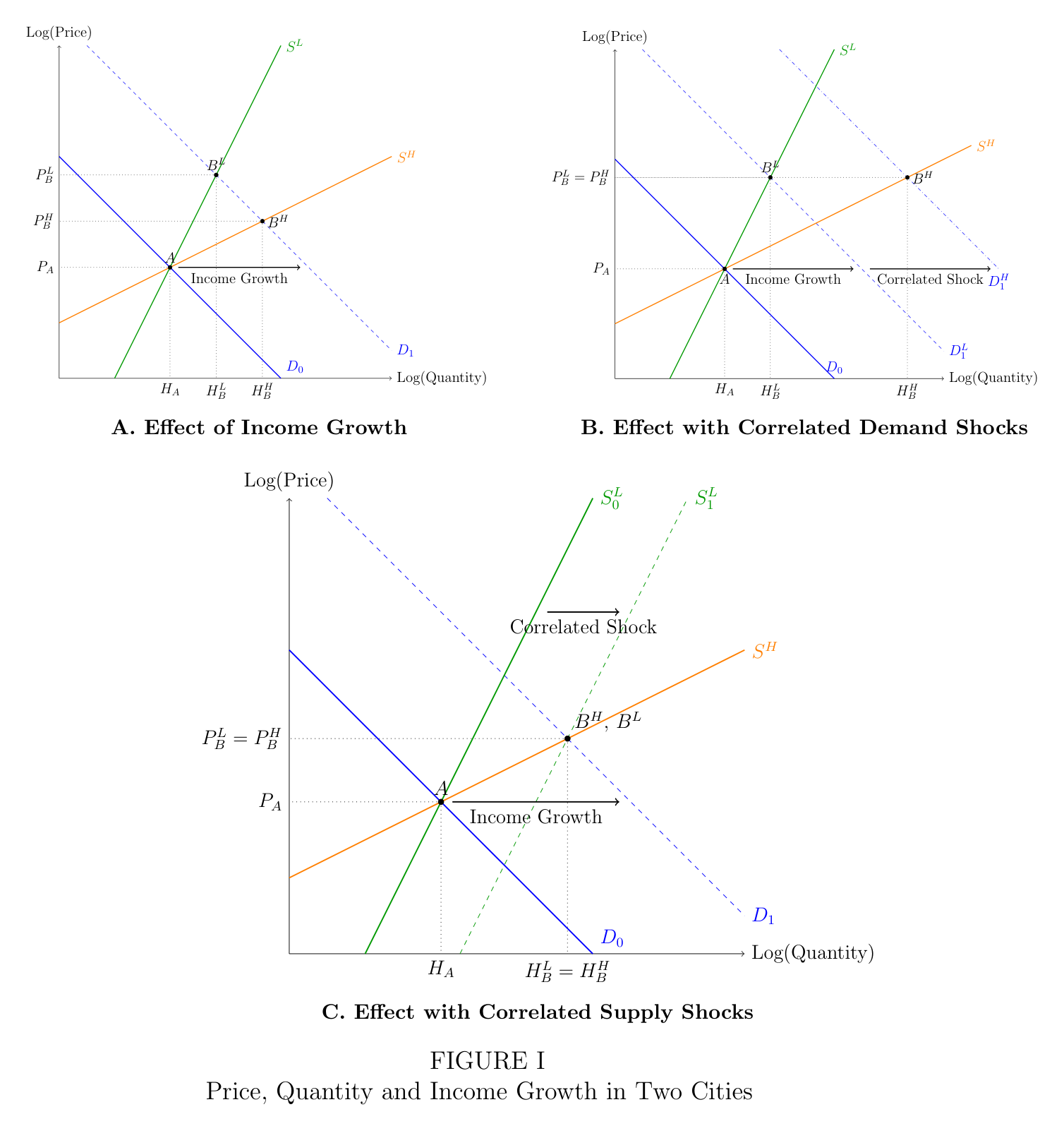
The authors lay out the canonicalAziz’s noteUgh. "Canonical" is, to me, some combination of AI slop and finance bro speak. view. Supply elasticity is the number at the center of everything: how much additional housing a city produces when prices rise. By this reading, constrained cities (low elasticity) can't convert demand into homes, so demand becomes price; permissive cities (high elasticity) convert it into construction, so demand becomes homes.
At this point, don't get bogged down in those chartsAziz’s noteNot trying to boss you around, dear reader—it's just that we will come back to panels B and C in a sec.... For now, just focus on panel A—it merely illustrates a normal supply-demand situation, where amid a shift out in the demand curve, the observed change in price tells you how elastic the supply curve is. This is the basis for the whole paper.
Using four standard measures of housing supply elasticities/constraints from the literature, we find that in response to higher income growth from 2000–2020 cities measured as having more elastic housing supply show the same growth in house prices, quantities, population, rents, commuting times, and rooms per person as cities measured as having less elastic housing supply. This is true across all the measures of housing constraints that we use, if we extend our sample to 1980, if we separate income growth into per capita income growth or population growth, and if we use plausibly exogenous changes in housing demand driven by standard instruments in the literature or exposure to pandemic-era work-from-home. In short, estimated housing supply constraints do not explain differences in house price and quantity growth across cities.
As stated in abstract.
Although the majority of our estimates are explicitly non-causal, in Section 2 we provide four arguments that they accurately quantify the (negligible) differences in actual housing supply elasticities across cities, at least as captured by these measures. First, if city income growth is uncorrelated with city supply shocks σ̂, then our estimates identify the true group-specific supply elasticities ψ, where j ∈{L, H} denotes the inelastic (L) and elastic (H) cities regardless of unobserved demand shocks. Intuitively, income growth will move house prices and quantities along the group-specific supply curve Ĥ = ψ P̂ and thereby identify the group-specific supply elasticity ψ from the co-movement of quantities and prices. Even if population growth, and therefore income growth, responds differently to demand shocks in inelastic and elastic cities because of their different supply elasticities, this does not threaten identification as house prices and quantities continue to comove along the group-specific supply curve. Of course, it is well known that any variation in house price or quantity driven by demand is sufficient to identify a supply elasticity (Angrist and Krueger, 2001Instrumental Variables and the Search for Identification (JEP 2001)The methods classic both sides cite: demand-side variation, even messy, can trace out a supply curve—the instrument need only be uncorrelated with supply shocks.Paper →; Saiz, 2010The Geographic Determinants of Housing Supply (QJE 2010)The field's standard supply-elasticity estimates: satellite measures of water and steep slopes, combined with regulation, yield an elasticity for every metro. Miami, LA, SF, NY, Boston, Chicago and Seattle rank among the most inelastic; Houston, Austin, Charlotte, Kansas City and Indianapolis among the most elastic.Paper →).
Second, if supply shocks σ̂ are correlated with income growth, our estimates still reflect relative differences in supply elasticities, provided this correlation is uniform across cities. The comovement of house price growth and quantity growth conditional on income growth will then identify the supply elasticity ψ and a bias term, with the size of the bias corresponding to the correlation between supply shocks and income growth. If those supply shocks are equally important in inelastic and elastic cities, our estimates will still identify the relative supply elasticity ψ −ψ across cities as the bias is “differenced” out. So even the presence of unobserved supply shocks is not a problem for our analysis. However, a plausible prior derived from a standard housing production function actually suggests that supply shocks should be less important in inelastic areas, consistent with the notion that quantities vary less in these markets. This prior implies that our estimates should be biased towards finding even larger differences in supply elasticities when they exist. In order for our estimates to obscure genuine differences in supply elasticities, supply shocks would instead need to be more correlated with income growth in cities classified as inelastic.
Third, even if one is willing to assume that supply shocks are more strongly correlated with income growth in inelastic cities, our results could only be explained by a highly specific scenario, one which contradicts conventional wisdom about housing supply elasticities. Specifically, the stronger correlation could occur either because supply shocks are more positively correlated with labor demand shocks or because supply shocks are relatively more important in inelastic cities. Within a standard spatial equilibrium framework (Moretti, 2011Local Labor Markets (Handbook chapter, 2011)The standard framework for how workers move between cities in response to wages, amenities and housing costs—the model class in which migration can equalize price-to-income ratios.Paper →), the hypothesis that supply shocks are relatively more important implies additional correlations that are clearly rejected by the data: it predicts substantial differences in how house prices and quantities comove with per capita income growth in more- and less-elastic cities. But the correlations between both house price and quantity growth with per capita income growth are indistinguishable across the groups of cities, clearly rejecting this hypothesis. Therefore, the only remaining scenario is that supply shocks systematically correlate more strongly with labor demand shocks in inelastic cities. Under this scenario, inelastic cities experiencing substantial per capita income growth (such as San Francisco) would need to consistently achieve relative productivity improvements in construction compared to elastic cities with similar per capita income growth (such as Austin), precisely offsetting any genuine elasticity differences. We are unaware of any literature proposing such a specific scenario persisting over the last four decades. Moreover, even if such conditions held, it would still imply that differences in supply elasticities do not explain differences in house prices and quantities across cities.
Fourth, our causal estimates, generated from both well-established instrumental variables and recent remote work shocks, give the same results: existing measures of housing supply constraints do not explain differences in house price and quantity growth across cities. Because these instruments plausibly isolate shifts in housing demand that are uncorrelated with supply-side shocks, they are not subject to the deus ex machina explanation above. The fact that these estimates give the same results as our non-causal estimates reinforces our interpretation of the non-causal estimates, suggesting that any genuine differences in housing supply elasticities are small or, if they do exist, are not captured by these widely used measures.
In summary, the simplest and most coherent interpretation of our findings is that standard measures of housing supply elasticities do not reflect actual differences in housing supply elasticities across cities, either because genuine differences are negligible or because they are measured with significant error. If measurement error is the explanation for our results, then that raises the question whether one can measure supply constraints across cities in an actionable way for policy decisions. Because each of the constraint measures we use is estimated in a fundamentally distinct way, it is unlikely that they are all subject to the same measurement error. Instead, it is more plausible that genuine supply elasticity differences are small. Critically, our results do not imply that supply “doesn’t matter.” Our framework assumes the fundamental and correct premise that exogenous expansions in housing supply will expand quantities and reduce prices; equivalently, we assume that supply curves slope up and demand curves slope down at the MSA level.
As with most economics papers, the findings here come from a regression—a line fit through points on a scatter plot. Economists call this non-causal evidence and are trained to approach it skeptically, because correlation is not causation.
For this paper specifically, non-causality raises several potential problems. The authors address three of them up front, and argue none should undermine their findings.
Potential problem 1: what if there is unobserved demand that systematically travels with measured income growth in one group of cities (panel B above)? Then a rise in price would get interpreted as lying along an inelastic supply curve when it really lies along an elastic one. The authors' defense: if this were a real problem here it would be obvious, because the same hidden demand would produce an outsized quantity response in those cities. The quantity data shows none.
Potential problem 2: what if there are hidden supply shifts that travel with measured income growth? The authors argue that as long as those shifts hit constrained and unconstrained cities alike, they cancelAziz’s noteA standard model of homebuilding implies the shifts should matter more where building is easy—which would bias the comparison toward finding differences between cities, the opposite of the null they find. when the two groups are compared.
Potential problem 3: what if supply shifts really did favor the constrained cities, ie that NIMBY cities really do have inelastic supply, just that it's been shifting out over time in a way that obscures how inelastic their supply curves are (panel C above)? To produce these results, San Francisco would need construction-productivity windfalls that precisely offset its rigidity, decade after decade, leaving it indistinguishable from Austin—and this coincidence would have to hold across every constrained city at onceAziz’s noteEven if the coincidence held, it would still mean elasticity differences don't explain the outcomes—the outcomes would be identical across cities either way.. "We are unaware of any literature proposing such a specific scenario persisting over the last four decades."
The authors also point out that where they do have causal variation—standard instruments and the pandemic remote-work shock—the answer comes out the same.
We next describe our results in more detail. Our empirical analysis uses four measures of housing supply constraints which have been very influential or represent the cutting edge of research in the area. These are the foundational supply elasticity from Saiz (2010)The Geographic Determinants of Housing Supply (QJE 2010)The field's standard supply-elasticity estimates: satellite measures of water and steep slopes, combined with regulation, yield an elasticity for every metro. Miami, LA, SF, NY, Boston, Chicago and Seattle rank among the most inelastic; Houston, Austin, Charlotte, Kansas City and Indianapolis among the most elastic.Paper →, a supply elasticity from Baum-Snow and Han (2024)The Microgeography of Housing Supply (JPE 2024)Modern supply-elasticity estimates built from neighborhood-level data—one of LMW's four constraint measures.Paper →, the Wharton Residential Land Use Regulation Index (WRLURI) from Gyourko, Saiz and Summers (2008)The Wharton Residential Land Use Regulation Index (Urban Studies 2008)The WRLURI: a national survey of municipal land-use regulation—approval delays, lot-size rules, growth controls—aggregated into the standard index of how regulated each market is.Paper →, and the land share of value from Davis, Larson, Oliner and Shui (2021)The Price of Residential Land for Counties, ZIP Codes, and Census Tracts (Journal of Monetary Economics 2021)Land price and land-share estimates for every county, ZIP and tract, built from appraisals of land 'as-is'—the source of LMW's fourth constraint measure.Paper → (Section 3). We use the terms “housing supply constraint” and “housing supply elasticity” interchangeably to describe these measures.
In our benchmark analysis in Section 4, we regress house price growth and house quantity growth on total income growth, an indicator if the city’s housing supply is measured as relatively less constrained (more elastic), and the interaction of income growth and the constraint indicator. We use total income growth to capture the net of changes in both average income and population as both margins reflect housing demand, but we also examine each component separately and find the same results. Total income growth is strongly correlated with growth in house prices, but the interaction of income growth with the constraint is economically and statistically insignificant across all of the measures. In other words, differences in income growth predict the same differences in house price growth in cities measured to be more or less constrained. We turn to housing quantities and find the same results: income growth is strongly correlated with growth in the number of housing units and growth in population, but this correlation is not affected by any of the measures of housing supply constraints. We make this point explicit by leveraging the comovement of prices and quantities and estimating an instrumental variable specification to recover the elasticities of housing quantities to prices for more- and less-constrained cities. Our estimated elasticities are all around one and, critically, are statistically and economically indistinguishable across cities measured to be relatively more or less constrained.
There are many ways to measure how hard it is to build in a city, and the authors use four of them: Saiz's geography-based elasticities (the field's workhorse, built from satellite measurements of steep slopes and water), a newer elasticity estimate from Baum-Snow and Han, the Wharton Residential Land Use Regulation Index (a survey of how demanding each metro's approval process is), and the land share of home value. Why use 4? Because they were built by different researchers from entirely different raw material—geography, surveys, appraisals—even if some of these don't measure constraints perfectly, they together should give an unbiased picture of constraints.
Then the benchmark regression, which everything else in the paper elaborates: regress price growth (and separately, quantity growth) on income growth, an indicator for being less constrained, and the interactionAziz’s noteThis is the key measure: do supposedly easy-to-build-in cities differ meaningfully from supposedly hard-to-build-in ones? Eg, do they build more amid higher demand, and do their prices rise less? of the two.
As discussed above, if these results are explained by a greater importance of supply shocks in inelastic cities then specifications using per capita or population growth should give different results. Instead we find that growth in per capita income and population both have identical correlations with house price and quantity growth in more- and less-constrained cities. We also examine growth in rents, the change in the average number of rooms per person, and the change in average commuting times and find that elastic and inelastic cities all exhibit the same correlation with income growth. We extend our sample to 1980 and find the same results when looking at growth from 1980 to 2000 or from 1980 to 2020. We explore finer discretizations of the constraint measures and continuous interaction models, all with the same results. The fact that measured constraints do not affect the correlations of house price or quantity growth with income growth is a robust feature of the data for at least the 40 years from 1980 to 2020.
To maintain that supply elasticities are nevertheless different in the face of our evidence requires believing that housing supply shocks must be more positively correlated with labor demand shocks in inelastic cities. This implies that high-growth, inelastic cities have benefited from positive supply shocks that exactly nullified the impact of a lower supply elasticity. We are not aware of anyone in the literature making this claim, which is also inconsistent with the claim that supply constraints are important in explaining house price growth and housing quantity growth across cities.
A much simpler interpretation of our results is that supply elasticities are either similar across cities or genuine differences are not captured by existing measures. Our results using exogenous housing demand shock are also consistent with this view. First, we employ standard instruments from the literature (see Saiz (2010)The Geographic Determinants of Housing Supply (QJE 2010)The field's standard supply-elasticity estimates: satellite measures of water and steep slopes, combined with regulation, yield an elasticity for every metro. Miami, LA, SF, NY, Boston, Chicago and Seattle rank among the most inelastic; Houston, Austin, Charlotte, Kansas City and Indianapolis among the most elastic.Paper →, Diamond (2016)The Determinants and Welfare Implications of US Workers' Diverging Location Choices (AER 2016)Cities attracting educated workers develop better amenities endogenously—the mechanism by which rising demand makes places nicer, which price indexes then record as price growth.Paper →, and Chodorow- Reich, Guren and McQuade (2024)The 2000s Housing Cycle with 2020 Hindsight (Review of Economic Studies 2024)Revisits the 2000s boom-bust with twenty years of hindsight: the cities that boomed and busted ended up with the highest prices by 2020, pointing to fundamentals-driven demand. LMW borrow its demand instruments—a supersector Bartik shock and climate.Paper → among many others), a Bartik shock and local climate measures, in our baseline sample. Using these instruments recovers estimates of average supply elasticities in line with the literature, but we find no evidence that elasticities are relatively larger in cities measured as more elastic compared to ostensibly less-elastic cities. Second, we rely on the literature documenting the effect of remote work on housing demand (Howard, Liebersohn and Ozimek, 2023The Short- and Long-Run Effects of Remote Work on U.S. Housing Markets (Journal of Financial Economics 2023)Remote work raised housing demand and prices in both the short and long run by moving demand across cities—the same class of shock LMW use for their causal check.Paper →; Mondragon and Wieland, 2025Housing Demand and Remote Work (NBER WP)Establishes pre-pandemic remote-work exposure as a valid, plausibly exogenous shifter of post-2020 housing demand—the instrument behind LMW's cleanest causal test.Paper →) and check if the shift to remote work or work from home (WFH) had differential effects from 2019 to 2023 depending on the measured housing constraints. Consistent with prior research, we find that exposure to WFH caused an increase in housing demand and house prices. Critically, the increase in house prices was essentially identical regardless of whether the city was more or less constrained. Similarly, exposure to WFH caused large increases in the growth of units permitted for construction and, conditional on the same exposure to WFH, cities saw similar growth in permitted units regardless of the measure of housing supply constraints. Despite these estimates coming from an out-of-sample period of exceptional economic changes and the distinct source of variation, we find the same results as in our baseline analysis, further validating the view that supply elasticities are not truly different across cities or that they are different but these differences have not yet been measured well.
Most of this section is an elaboration on the points above: re why non-causal estimates aren't a problem here (they add more evidenceAziz’s noteRecall that one worry with the regressions is that income growth might be tangled up with a city's supply conditions (ie, the case where a NIMBY city seems to make it easy to build but where the reality is they make it hard to build, and are merely simultaneously benefitting from positive supply shocks, eg technology).
So they rerun the regression using a measure of demand that—unlike their primary measure (total income growth, which is additional population timex additional income)—can't be correlated with supply.
One source is a "Bartik shock": a city's predicted demand boom based on which industries it started with and how those industries later grew nationally—a city that happened to specialize in software got a demand surge from the national rise of software, not from anything about its own housing market.
The other is climate—January temperature and July humidity—since people persistently migrate toward mild winters, and a city's weather can't be caused by its zoning.
These instruments produce sensible average supply elasticities, in line with the standard published numbers, but still show no difference between the supposedly constrained and unconstrained cities.).
Then they talk about how to interpret the results.
The simplest interpretation, the authors write, is that supply elasticities are “either similar across cities or genuine differences are not captured” by the standard measures.
I think what's important here is that, even if that latter is true, and the 4 measures of "hard to build" (for example due to zoning restrictions) don't correctly capture the reality of how hard it is to build, this doesn't redeem the YIMBY framework, since the edifice of evidence supposedly in favor of regulation-as-cause-of-high-home-prices argument is also based on these measures.
Here is where I got a bit confused with semantics—especially the use of "demand". If you're like me, rollover thisAziz’s noteNote the two meanings of "demand": the demand curve (on a price-quantity chart) and the demand shifter: income growth, the push that moves that demand curve.
The x-axis, and all the worry about demand correlating with supply, is about the shifter: was the push a city got related to its supply side?
(how could this happen? Imagine a booming city uses its swelling tax base to build highways and sewer lines into surrounding farmland. The income growth and an outward supply shift arrive together—the same boom that pushed demand also opened land to development)..
But if not supply constraints, how do we explain that house prices have grown more and housing quantities have grown less in San Francisco compared to Houston—two poster-children of ostensibly different supply elasticities. In Section 5, we propose that housing markets feature both quantity (units) and quality (location, finishes, size, and so on) margins and that cities can experience different demand shifts along these margins. Intuitively, increases in per capita income will tend to increase the demand for housing quality with little effect on the demand for units, while increases in population (driven by growth in employment, for example) will tend to increase the demand for housing units. This implies that the comovement of prices, quality, and quantities will depend critically on the composition of demand shifts. For example, a housing demand shock for quality will raise house prices without raising quantities, making unit supply look inelastic irrespective of the underlying unit supply elasticity. Consistent with this model, per capita income growth and population growth yield very different estimates of housing supply elasticities, and the differences in house price growth and housing quantity growth across San Francisco and Houston can be largely explained by their differences in per-capita income and population growth.
In short, we establish that measures of local housing supply constraints do not help us understand how shifts in demand translate into house price and quantity growth across U.S. cities. This finding challenges the standard view that supply constraints explain rising house prices across cities and suggests that efforts to relax measured housing constraints may have negligible effects on house prices and quantities. Instead we propose that the composition of housing demand is a currently underappreciated but potentially critical factor for understanding differences in housing dynamics across cities.
I think one challenge in interpreting this paper is that it runs so contrary to intuition. To their credit, the authors recognize this and address it head-on.
Take San Francisco and Houston. The two cities experienced almost identical growth in total demand but had very different outcomes: Houston built far more, and its prices rose far less.
At first glance this seems to flatly contradict the paper's finding—that NIMBY and YIMBY cities respond the same way, in building and in prices, to rising demand.
But here's the key, and I don't think the paper makes it clear enough: their finding is about group averages, and these two cities lie off the trend lines. Given its demand, SF built less and saw prices rise more than the typical NIMBY city; Houston built more than the typical YIMBY city. Neither is representative of its group.
So the authors are saying: a typical NIMBY city and a typical YIMBY city facing the same total demand would have built the same amount and seen nearly the same additional price growth. SF and Houston are just not typical—they didn't behave like their broader groups (YIMBY, NIMBY cities).
But what makes them atypical? Why did they deviate so much from how other cities in their groups responded? The authors argue it's the composition of their demand: San Francisco's arrived almost entirely as rising incomes, Houston's as rising population.
The preview of Section 5, where they explain that "demand" is really two different things: demand for more units (you see this in a place like Houston with growing population) and demand for better units (you see this in a place like SF with a stagnant population but rising incomes).
Housing supply constraints are now generally agreed to be an important, if not the most important, impediment to affordable housing (Glaeser, Gyourko and Saks, 2005Why Have Housing Prices Gone Up? / Urban Growth and Housing Supply (2005-06)Founding papers of the regulation view: house prices increasingly exceed construction costs in regulated markets, and the gap is attributed to regulatory barriers—the 'regulatory tax.'Paper →; Saiz, 2023The Geographic Determinants of Housing Supply (QJE 2010)The field's standard supply-elasticity estimates: satellite measures of water and steep slopes, combined with regulation, yield an elasticity for every metro. Miami, LA, SF, NY, Boston, Chicago and Seattle rank among the most inelastic; Houston, Austin, Charlotte, Kansas City and Indianapolis among the most elastic.Paper →). Gyourko (2009)Housing Supply (Annual Review of Economics 2009)A survey of housing supply research: what is known about the technology, elasticities and regulation of homebuilding.Paper →, Gyourko and Molloy (2015)Regulation and Housing Supply (Handbook of Regional and Urban Economics 2015)The Handbook survey of land-use regulation: what it is, how it is measured, and the evidence that it constrains construction and raises prices.Paper →, Glaeser and Gyourko (2018)The Economic Implications of Housing Supply (JEP 2018)The consensus statement: regulation drives a wedge between prices and construction costs in coastal markets, with broad economic costs.Paper →, and Molloy (2020)The Effect of Housing Supply Regulation on Housing Affordability: A Review (RSUE 2020)Raven Molloy's survey of the regulation literature. It concludes that regulation raises house prices, but that the evidence on affordability for low-income households is thinner and more mixed than the confidence of the policy debate suggests—one of the four surveys LMW cite as defining the consensus they test.Paper → provide surveys of this extensive literature. A common theme is that supply elasticities are not uniform across U.S. cities. Gyourko, Saiz and Summers (2008)The Wharton Residential Land Use Regulation Index (Urban Studies 2008)The WRLURI: a national survey of municipal land-use regulation—approval delays, lot-size rules, growth controls—aggregated into the standard index of how regulated each market is.Paper → and Gyourko, Hartley and Krimmel (2021)The Local Residential Land Use Regulatory Environment Across U.S. Housing Markets (JUE 2021)The updated Wharton regulation index, from a 2018 survey—evidence on how the regulatory environment varies across and within US markets.Paper → developed indexes of regulatory constraints that ostensibly reduce supply elasticities across different metropolitan entities. Saiz (2010)The Geographic Determinants of Housing Supply (QJE 2010)The field's standard supply-elasticity estimates: satellite measures of water and steep slopes, combined with regulation, yield an elasticity for every metro. Miami, LA, SF, NY, Boston, Chicago and Seattle rank among the most inelastic; Houston, Austin, Charlotte, Kansas City and Indianapolis among the most elastic.Paper → recovered MSA-level elasticities incorporating geographic and regulatory constraints to show that metros with little developable land due to geographic constraints from water bodies or steep terrain are the very places often deemed to have inelastic housing supply. Baum-Snow and Han (2024)The Microgeography of Housing Supply (JPE 2024)Modern supply-elasticity estimates built from neighborhood-level data—one of LMW's four constraint measures.Paper → estimate supply elasticities at the census tract level and trace out how the supply response across the metro area varies with geographic and regulatory constraints. Davis, Larson, Oliner and Shui (2021)The Price of Residential Land for Counties, ZIP Codes, and Census Tracts (Journal of Monetary Economics 2021)Land price and land-share estimates for every county, ZIP and tract, built from appraisals of land 'as-is'—the source of LMW's fourth constraint measure.Paper → use a large micro dataset to estimate the land share of value, which indicates the relative tightness of housing supply constraints in a class of models (Glaeser and Gyourko, 2003The Impact of Building Restrictions on Housing Affordability (FRBNY Economic Policy Review 2003)The original 'regulatory tax' paper: where house prices exceed construction costs, the gap is attributed to building restrictions. The method Murray (2021) and O'Flaherty later criticized.Paper →), across a large variety of geographies. Additional papers estimating local housing supply constraints or elasticities in the U.S. include Green, Malpezzi and Mayo (2005)Metropolitan-Specific Estimates of the Price Elasticity of Supply of Housing (AER P&P 2005)An early catalog of metro-specific housing supply elasticities, documenting enormous variation across markets.Paper →, Glaeser, Gyourko and Saks (2005)Why Have Housing Prices Gone Up? / Urban Growth and Housing Supply (2005-06)Founding papers of the regulation view: house prices increasingly exceed construction costs in regulated markets, and the gap is attributed to regulatory barriers—the 'regulatory tax.'Paper →, Davis and Palumbo (2008)The Price of Residential Land in Large US Cities (JUE 2008)Constructs land price series for large US cities, showing land's share of home value rising sharply over recent decades, especially on the coasts.Paper →, Kok, Monkkonen and Quigley (2014)Land Use Regulations and the Value of Land and Housing (JUE 2014)Intra-metropolitan evidence from the San Francisco Bay Area that land use regulation raises the value of land and housing at fine geography.Paper →, Gorback and Keys (2020)Global Capital and Local Assets (NBER WP 2020)Uses foreign capital inflows as a housing demand shock to estimate house price and quantity elasticities across US markets.Paper →, Albouy and Stuart (2020)Urban Population and Amenities: The Neoclassical Model of Location (International Economic Review 2020)Calibrates the neoclassical location model to US cities, quantifying how amenities, productivity and land constraints jointly determine urban populations and prices.Paper →, Guren, McKay, Nakamura and Steinsson (2021b)Housing Wealth Effects: The Long View (Review of Economic Studies 2021)Estimates metro-level housing wealth effects over four decades, producing house-price sensitivities to local demand—part of the literature relating price responses to supply constraints.Paper →, and Chodorow-Reich, Guren and McQuade (2024)The 2000s Housing Cycle with 2020 Hindsight (Review of Economic Studies 2024)Revisits the 2000s boom-bust with twenty years of hindsight: the cities that boomed and busted ended up with the highest prices by 2020, pointing to fundamentals-driven demand. LMW borrow its demand instruments—a supersector Bartik shock and climate.Paper →. For a review of international evidence on housing supply elasticities see Saiz (2023)The Geographic Determinants of Housing Supply (QJE 2010)The field's standard supply-elasticity estimates: satellite measures of water and steep slopes, combined with regulation, yield an elasticity for every metro. Miami, LA, SF, NY, Boston, Chicago and Seattle rank among the most inelastic; Houston, Austin, Charlotte, Kansas City and Indianapolis among the most elastic.Paper →.
In addition to potentially driving up house prices, tight housing supply has been linked to pernicious effects on other important economic outcomes. Saks (2008)Job Creation and Housing Construction (JUE 2008)Metros with less housing supply see smaller employment gains and larger price increases after labor demand shocks—an early estimate of regulation's wider economic costs.Paper →, Paciorek (2013)Supply Constraints and Housing Market Dynamics (JUE 2013)A dynamic model in which regulation raises both the level and volatility of house prices by slowing the supply response to demand shocks.Paper →, Gyourko, Mayer and Sinai (2013)Superstar Cities (AEJ: Economic Policy 2013)A few scarce, desirable cities capture growing numbers of high-income households, whose bidding drives long-run price divergence—demand concentrating on fixed places.Paper →, Ganong and Shoag (2017)Why Has Regional Income Convergence Declined? (JUE 2017)Argues housing constraints broke the century-old pattern of poor states catching up to rich ones, by pricing low-skill workers out of high-income places.Paper →, Gaubert (2018)Firm Sorting and Agglomeration (AER 2018)More productive firms sort into larger cities; the calibrated model quantifies how policies that distort city sizes—housing constraints among them—affect aggregate output.Paper →, and Hsieh and Moretti (2019)Housing Constraints and Spatial Misallocation (AEJ: Macro 2019)The famous misallocation estimate: housing constraints in high-productivity cities lowered aggregate US growth by keeping workers out of the most productive places. A pillar of the supply-centric consensus LMW challenge.Paper →, among others, argue that differences in housing supply elasticities have important effects on outcomes ranging from housing market volatility to aggregate productivity. Been, Ellen and O’Regan (2019)Supply Skepticism: Housing Supply and Affordability (Housing Policy Debate 2019)The 'supply skepticism' survey: reviews the evidence that adding market-rate supply improves affordability and responds to the skeptics who doubt it.Paper → surveys work linking supply restrictions to environmental costs, segregation, and inequality. Glaeser and Gyourko (2018)The Economic Implications of Housing Supply (JEP 2018)The consensus statement: regulation drives a wedge between prices and construction costs in coastal markets, with broad economic costs.Paper → also provide a survey and discussion on the broader costs of tight housing supply.
There is a growing literature that examines the local effects of new construction on outcomes like neighborhood rents and demographic composition. Examples include Zahirovich- Herbert and Gibler (2014)The Effect of New Residential Construction on Housing Prices (Journal of Housing Economics 2014)Estimates how new residential construction changes the sale prices of nearby existing homes—one of the neighborhood-level studies LMW cite on local price effects.Paper →, Diamond and McQuade (2019)Who Wants Affordable Housing in Their Backyard? (JPE 2019)Equilibrium analysis of LIHTC development: affordable housing projects raise surrounding property values in low-income neighborhoods and lower them in high-income ones.Paper →, Pennington (2021)Does Building New Housing Cause Displacement? (working paper 2021)Uses San Francisco building fires as natural experiments: new construction lowers nearby rents and reduces displacement—quasi-experimental evidence that new supply helps its neighborhood.Paper → and Li (2022)Do New Housing Units in Your Backyard Raise Your Rents? (Journal of Economic Geography 2022)New market-rate towers in New York lower nearby rents through added supply, partly offset by amenity effects as new businesses follow.Paper →. Some, although not all, of these papers find evidence that new construction reduces rent growth in the affected area. These estimates, by studying shifts in local housing supply, identify the shape of the local demand curve. By contrast, our approach identifies the slopes of the city-level supply curves in more- and less-constrained cities, which is critical for understanding the extent to which supply constraints affect housing affordability. Therefore, our results are not in conflict with these papers. A more closely related body of work studies changes in zoning constraints and how this affects the supply of housing, which should be informative about how much the housing supply function is affected by regulatory constraints. This work is surveyed by Freemark (2023)Zoning Change (Journal of Planning Literature 2023)Surveys studies of actual zoning reforms—upzonings and downzonings—and reports mixed, generally modest effects on construction and prices. The closest evidence to a direct test of what deregulation does.Paper →, who reports mixed and generally modest effects of zoning changes on housing prices or quantities, consistent with our results.
A number of other studies have also found a limited role for supply elasticity differences in the cross-section of U.S. cities. Rodríguez-Pose and Storper (2020)Housing, Urban Growth and Inequalities (Urban Studies 2020)The influential critique of deregulation from economic geography: upzoning is unlikely to improve affordability or reduce inequality; income growth, not regulation, drives prices.Paper → give an influential critique of the idea that relaxing regulatory barriers is likely to improve affordability, reduce inequality, or spur growth and also make the argument that income growth drives house prices. Similarly, Buchholz, Kemeny, Randolph and Storper (2026)Inequality, Not Regulation (working paper 2026)Argues the affordability crisis traces to income inequality rather than land-use regulation—the inequality school's most direct statement.Paper → argue that inequality, not regulation, is the source of the “affordability crisis.” Davidoff (2013)Supply Elasticity and the Housing Cycle of the 2000s (Real Estate Economics 2013)The 2000s boom-bust was not larger in supply-inelastic regions once demand is accounted for; the regions with the biggest cycles also built the most.Paper → shows that regions with the largest 2000s housing cycle also saw the highest growth in quantities and that, conditional on demand, the amplitude of the 2000s housing cycle is not larger in less-elastic cities. Davidoff (2016)Supply Constraints Are Not Valid Instrumental Variables for Home Prices (Critical Finance Review 2016)Shows the standard constraint measures are 'correlated with many demand factors'—education, immigration, industry mix—so regulated coastal markets are expensive partly because they are desirable and productive, invalidating constraints as instruments.Paper → further finds that cities with lower measured supply elasticity experience both higher house price and quantity growth from 1980-2012 and argues that this reflects a negative correlation of supply elasticities with demand shocks. Like Davidoff (2013, 2016)Supply Elasticity and the Housing Cycle of the 2000s (Real Estate Economics 2013)The 2000s boom-bust was not larger in supply-inelastic regions once demand is accounted for; the regions with the biggest cycles also built the most.Paper → we jointly examine house prices and quantities, and show that OLS regressions interacting income with supply elasticities can help us determine the role of supply elasticities in explaining house price and quantity growth across cities.
Howard and Liebersohn (2021)Why Is the Rent So Darn High? (Journal of Urban Economics 2021)Builds a new rent index and finds the effect of income growth on rents is independent of measured supply elasticity, attributing this to strong migration responses—rising demand to live in inelastic cities drives rents everywhere.Paper → show that the effect of income growth on their newly-constructed rent index from 2000-2018 is independent of the measured housing supply elasticity, which they attribute to a high migration elasticity. Similarly, Aura and Davidoff (2008)Supply Constraints and Housing Prices (Economics Letters 2008)A calibrated model in which even large local supply expansions barely move prices, because migration and demand from outside the region absorb them—relaxing one city's constraints does little.Paper → and Anenberg and Kung (2020)Can More Housing Supply Solve the Affordability Crisis? (RSUE 2020)A calibrated neighborhood-choice model in which plausible supply expansions have small effects on rents—demand substitutes across neighborhoods.Paper → use quantitative calibrated models to argue that relaxing local housing supply constraints is unlikely to significantly affect local house prices due to strong migration responses. Molloy, Nathanson and Paciorek (2022)Housing Supply and Affordability (JUE 2022)Finds a weak relationship between supply elasticities and rents—the price of housing services—though larger effects on house prices and quantities.Paper → find a weak relationship between elasticities and rents, although they argue there are large effects on prices and quantities. Davis and Ortalo-Magné (2011)Household Expenditures, Wages, Rents (Review of Economic Dynamics 2011)Housing expenditure shares are roughly constant across cities and time—implying rents move with incomes and supply elasticities should be uncorrelated with rent levels.Paper → examine data on expenditure shares on housing for renters and find that these shares are constant across MSAs, concluding that supply elasticities will be uncorrelated with rents and prices. We depart from most of these papers by also showing that growth in housing quantities and population, not just house price growth, is independent of local supply elasticities, and thus infer a limited role for housing supply elasticities (and so migration induced by differential elasticities) in explaining the cross-section of U.S. city house price and quantity growth since at least 1980.
In his discussion (available here) of Glaeser and Gyourko (2003)The Impact of Building Restrictions on Housing Affordability (FRBNY Economic Policy Review 2003)The original 'regulatory tax' paper: where house prices exceed construction costs, the gap is attributed to building restrictions. The method Murray (2021) and O'Flaherty later criticized.Paper →, O’Flaherty lays out a number of important critiques of the single-margin housing model and related empirical approaches. In particular, he shows that when there are multiple margins of housing demand then it is very challenging to infer the marginal value of housing units and land. Murray (2021)Marginal and Average Prices of Land Lots Should Not Be Equal (Environment and Planning A 2021)Argues marginal and average land prices differ for basic economic reasons, undermining the Glaeser-Gyourko method of reading a regulatory tax off the gap between prices and construction costs.Paper → develops these critiques further. In Section 5 we extend this argument to show that higher demand for housing quality can be misinterpreted as inelastic housing supply.
These five paragraphs place the paper in the existing literature, and the choices reveal the strategy. Three groups of prior work get three different treatments.
The first group is the consensus under attack: the body of work linking tight supply to lost productivity, volatility, segregation, and inequality—Hsieh and Moretti's famous estimate that housing constraints cost the U.S. economy enormous amounts of output sits here. The authors don't engage it yet; they just name it as what their null threatens.
The second group looks like a contradiction and gets defused instead. A well-known micro literature finds that new buildings lower rents nearby. If building lowers rents, doesn't that prove supply matters? The authors' answer is a distinction that recurs throughout the paper: those studies shift supply and thereby trace out the demand curve—how prices respond when new units arrive. This paper compares supply curves across cities. Both can be true at once: building helps wherever it happens, and the constraint measures still fail to explain why cities differ. The genuinely comparable work—Freemark's survey of what happens when cities actually change their zoning—reports "mixed and generally modest effects," which the authors record as consistent with their null.
The third group is allies, and it is longer than most readers expect: Rodríguez-Pose and Storper's critique of deregulation, Buchholz and coauthors on inequality as the driver, Davidoff's two papers showing constraint measures tangled up with demand, Howard and Liebersohn finding rent growth independent of elasticity, Aura and Davidoff's calibrated models where migration neutralizes local supply differences. The claimed advance over all of them: adding quantities and population to the test. Price-only evidence leaves alternative explanations open—migration stories, measurement stories—and watching the building margin closes them.
The last paragraph names the paper's ancestors: O'Flaherty's old critique of Glaeser and Gyourko's regulatory-tax method, developed further by Murray—the argument that with multiple margins of housing demand, standard inferences about land and units break down. Section 5 is that critique, formalized. Readers of the Great Debate will recognize nearly every name on this page; the paper is consciously assembling one side of an existing war.
Using a standard demand-and-supply framework for the housing market, we demonstrate that non-causal OLS regressions predicting city-level house price and quantity growth from income growth interacted with the local supply elasticity inform whether differences in supply elasticities are important in explaining cross-city differences in house price growth and housing quantity growth.
We assume there are I cities indexed by i, each with a population N where individuals receive income y so that total income in the city is given as Y = yN and the total quantity of housing is H, purchased at the price P. For simplicity, we assume H is a measure of total housing consumption that encompasses both the extensive and intensive margins. In our empirical work we examine measures of both margins. Households also have some additional demand shifters θ, which can increase or decrease their demand for housing. These can be thought of as changes in the demand for amenities or changes in wealth (for example, stock market investments) that affect housing demand in the city. Therefore housing demand in the city is given by a general Marshallian demand function H = f(Y, P, θ). We linearize this expression to get the change in housing demand where hats indicate the percentage change and ϵ gives the relevant demand elasticity:
This housing demand function nests the demand functions from standard spatial equilibrium models. Consider the case in which households in location i earn y to spend on tradable non-housing goods c and nontradable housing h with relative price P. Under Cobb-Douglas preferences with housing share α (consistent with Davis and Ortalo-Magné, 2011Household Expenditures, Wages, Rents (Review of Economic Dynamics 2011)Housing expenditure shares are roughly constant across cities and time—implying rents move with incomes and supply elasticities should be uncorrelated with rent levels.Paper →), housing demand is h = α y P ⇒ H = hN = α Y P . In this model ϵ = 1, ϵ = 1, and θ̂ = α̂.
Our housing demand function (2) does not restrict the correlations between the demand shifter ˆθ and prices and income in any way. Intuitively, we can allow for arbitrary correlations of residual demand θ̂ with Ŷ and P̂ because any variation in demand that is correlated with income is valid variation for identifying relative supply curves. For this reason our demand function also nests intertemporal as well as spatial equilibrium models of housing demand (see Section A1).
Zoom all the way out first. The paper's question is: given the same demand, do cities respond differently? This section is the groundwork for answering that with data, and the whole pipeline looks like this:
Here is the problem the groundwork solves. The paper's main regression predicts a city's home price growth from its income growth, and it produces a coefficient of about 0.5: one extra point of income growth comes with about half a point of extra price growth. But that number is a blend. It mixes together the thing the debate is about (how much building a city produces when prices rise, the supply elasticity ψ) with things the debate is not about (how strongly households respond to income and to prices, and the influence of factors the data never measures). Until you know exactly what is in the blend, you cannot interpret the number, and you certainly cannot conclude anything from it being equal in NIMBY and YIMBY cities. Working out the blend is what the equations on the left do.
You can take the three conclusions on faith and skip the algebra. First, the cross-city comparison is legitimate because households everywhere behave the same way: they spend a roughly constant quarter of income on housing, in every kind of city, decade after decade (Davis and Ortalo-Magné (2011)Household Expenditures, Wages, Rents (Review of Economic Dynamics 2011)Housing expenditure shares are roughly constant across cities and time—implying rents move with incomes and supply elasticities should be uncorrelated with rent levels.Paper →). So the demand ingredients of the blend are the same in both groups, and differences in the coefficient could only come from ψ. Second, most contamination turns out to be harmless. Demand that the income measure misses (amenities, wealth, expectations) pushes prices and building together, so it cannot fake the paper's result in both regressions at once. The only dangerous contamination is supply-side luck that lines up with demand, and that is where the paper aims all of its later defenses. Third, the most useful result: divide the building coefficient by the price coefficient and everything about demand cancels. The ratio equals ψ itself. That is why the paper always watches prices and quantities together.
A short glossary for the terms on the left: a "Marshallian demand function" is the textbook name for quantity demanded as a function of income and price; "Cobb-Douglas preferences with housing share α" means households spend the fixed fraction α of income on housing; "linearizing" means converting everything to percentage growth rates, which is what the hats over the letters mean.
One more design choice matters: the authors impose no restriction on how the demand shifters correlate with prices, incomes, or each other. Demand is allowed to be endogenous, co-determined with the housing market, contaminated by supply conditions, anything. That permissiveness is deliberate. The identification comes from the structure of the supply side, not from pretending demand is clean. When Salim Furth later attacks the paper for putting an equilibrium outcome, total income, inside the demand function (his "taqueria" argumentFurth (2025), Response“An analogy: number of sales at taquerias would be an excellent predictor of the number of tacos sold. But we wouldn't include it in the demand function for tacos.”Open in context →: sales predict demand but can't define it), this is the passage the authors point back to. Their replyLMW, Response to Furth“total income is a completely valid measure of demand in both the standard local labor market model and even in the specific extension suggested by Furth in his comment.”Open in context → builds the full version of the answer. The framework never claimed the demand measure was exogenous; it was built so it wouldn't have to be. A footnote states the minimal requirement plainly: total income need not be a comprehensive measure of housing demand. It need only be correlated with it.
We assume the total supply of housing H is competitive and determined by an elasticity parameter ψ and supply shocks σ so that H = P σ. The elasticity ψ reflects the flexibility of the local housing construction sector as determined by regulations, geography, and so on. We abstract from the importance of other factors like local labor costs or financing costs. Linearizing this expression gives the change in total supply as
The differences that we consider should be thought of as long-run differences, in practice 20 years or more. Housing construction is time consuming, so that in the short-run almost all supply curves are relatively inelastic regardless of the long-run supply curve elasticities (Guren, McKay, Nakamura and Steinsson, 2021aWhat Do We Learn from Cross-Regional Empirical Estimates in Macroeconomics? (NBER Macroeconomics Annual 2021)Methods paper on cross-regional regressions in macro. LMW cite it for the point that 20-year differences wash out short-run cyclical variation, whatever the long-run supply elasticities.Paper →). The long view also justifies a stock-based supply curve relative to a flow-based supply curve (DiPasquale and Wheaton, 1994Housing Market Dynamics and the Future of Housing Prices (JUE 1994)A stock-flow model where construction responds to price levels as well as changes—one of Furth's suggested reasons elasticity comparisons may miss regulation's effects.Paper →), although the long-run equilibrium in those frameworks is identical to our own.
The housing market clears so that the total change in housing quantities is equal to the change in the supply of housing and the change in housing demand:
Solving for prices gives an intuitive expression for the change in prices as a function of changes in demand coming from income and residual demand shocks or from shifts in supply:
The effect of changes in income on house prices depends on the elasticity of housing demand to income, but this effect will be mitigated to the extent that housing supply elasticities are high or if demand is very sensitive to changes in the price. Shifts in supply σ̂ or residual demand θ̂ affect house prices in a similar way.
Substituting for prices into the supply equation gives a reduced form expression for the change in housing quantities:
Here as ψ becomes smaller (less elastic) then the denominator becomes larger, reducing the size of the quantity response at the same time that the price response in Equation (4) is increasing. These expressions nest standard local labor market/spatial equilibrium models (see Section A1).
The supply side is one line: the quantity of housing supplied rises with price, scaled by the supply elasticity (the disputed number), plus a supply-shock term for changes in the ability to build, such as cheaper construction, new land, or a regulatory change. Markets clear: prices and quantities settle where supply meets demand.
The rest of the passage combines the demand equation and the supply equation into the two equations the whole paper estimates: price growth as a function of income growth, and quantity growth as a function of income growth. The term "reduced form" just means an equation written in terms of things you can observe. The conclusion to carry forward is this: every observable outcome in the paper is now an explicit function of the supply elasticity. If two groups of cities really have different supply elasticities, the difference has to show up in how their prices and quantities respond to income growth. That is what makes the later null result a statement about elasticities rather than an absence of evidence.
Now assume that there are two kinds of cities, those with high supply elasticities and those with low supply elasticities and denote the respective set of cities by Ω (high) and Ω (low). We have data on house prices, quantities, and the total change in income for each city. We can estimate the relationship between changes in total income and house prices and quantities within each set of cities Ω using the following regression where j ∈{H, L} indicates if the city is of a high- or low-elasticity type
Running these regressions within each set of cities will recover the following estimates:
If there is no omitted variable bias coming from unobserved demand and supply shocks then the second terms will fall out so that the regressions recover the effects of income growth on house prices and quantities as mediated by the income elasticity of demand for housing, the price elasticity of demand for housing, and the housing supply elasticity. If households across cities do not differ in their income or price elasticities, the pass-through from income growth into house prices will be lower in cities with more elastic housing supply:
Figure IA illustrates this standard demand and supply logic where B indicates the equilibrium for each type of city after the shift in demand from the initial equilibrium. Thus, a regression of house price growth on income growth within high-elasticity cities should recover a smaller coefficient β relative to the coefficient β from the same regression of house prices on income growth within low-elasticity cities. For the regression of housing quantity growth on income growth we expect a larger response in the more elastic cities, γ > γ.
This passage builds the actual test. Split cities into a more-constrained half and a less-constrained half using each constraint measure, then run the price regression and the quantity regression in each half. The standard view makes a definite prediction about the results: the constrained half should show a larger price response to income growth and a smaller quantity response. The figure draws that prediction so it is on the record before the data arrives: the same demand increase pushed into a rigid housing market produces more price growth and less building than the same increase pushed into a flexible one.
The passage also states the condition under which the regressions cleanly measure each group's true response: the unmeasured shocks must not be correlated with income growth in a way that differs between the groups. Whether that condition holds is the subject of the next passage, which is the most important part of the framework.
More generally, the ratio of the OLS estimators from the quantity and price regressions shows when the co-movement of quantity and prices with income growth is informative about a city’s supply elasticity, γ β = ψ + Cov(σ̂, Ŷ) Cov( P̂, Ŷ) , j ∈{H, L}. (7) This ratio is equivalent to the IV estimator of housing quantity growth on house price growth instrumented by income growth.
When supply shocks are uncorrelated with income growth Cov(σ̂, Ŷ) = 0, then the ratio of quantity to price effects identifies the supply elasticity ψ. In particular, we can allow for arbitrary correlations of income with other demand shocks and arbitrary differences in the parameters of the housing demand function (2). Any variation in demand helps identify the slope of the supply curve (Angrist and Krueger, 2001Instrumental Variables and the Search for Identification (JEP 2001)The methods classic both sides cite: demand-side variation, even messy, can trace out a supply curve—the instrument need only be uncorrelated with supply shocks.Paper →; Saiz, 2010The Geographic Determinants of Housing Supply (QJE 2010)The field's standard supply-elasticity estimates: satellite measures of water and steep slopes, combined with regulation, yield an elasticity for every metro. Miami, LA, SF, NY, Boston, Chicago and Seattle rank among the most inelastic; Houston, Austin, Charlotte, Kansas City and Indianapolis among the most elastic.Paper →). For example, Figure IB illustrates the case when high elasticity places have a relatively stronger correlation between income growth and other positive demand shocks. This correlation will generate a relatively high correlation between income and house price growth pushing β closer to β. But we should then see an even larger difference in quantities, as the same demand shocks will push up housing quantities even more in more elastic cities so that γ >> γ. Intuitively, any demand shock moves quantity and prices along the city-specific supply curve, so their relative movements identify the slope of the supply curve ψ.
When supply shocks are correlated with income, then we no longer identify a city’s supply elasticity, but the relative co-movement can still identify the relative supply elasticity if the bias is the same in elastic and inelastic cities: γ β −γ β = ψ −ψ + Cov(σ̂, Ŷ) Cov( P̂, Ŷ) −Cov(σ̂, Ŷ) Cov( P̂, Ŷ) Empirically, we find that the covariance between prices and income is nearly identical across elastic and inelastic cities Cov( P̂, Ŷ) = Cov( P̂, Ŷ). Thus, if the covariance between supply shocks and income growth is also the same across cities, then comparing the comovement of quantities and prices conditional on income across inelastic and elastic cities will identify their relative supply elasticities.
A reasonable prior about these covariances is that supply shocks are relatively more important in elastic areas, which implies that we will be biased to recovering even larger differences in supply elasticities. Assume perfect competition and a CES production function for housing Q = A[α ¯K + (1 −α)L ] where A is construction productivity, ¯K is fixed land, L is labor, and ξ is the elasticity of substitution. The supply curve is then Q̂ = ψ P̂ + (1 + ψ) Â −ψc W where the supply elasticity is ψ = ξ(1 −s )/s and s = 1− is the land share. The microfounded housing supply shocks ˆσ ≡(1+ψ) ˆA−ψ ˆW scale with the supply elasticity, consistent with the intuitive notion that quantities will vary less in places where it is harder to build. Thus, to the extent that supply elasticities are different across cities, we expect supply shocks to be relatively more important in elastic cities, Cov(σ̂, Ŷ) < Cov(σ̂, Ŷ), and our estimates would be biased towards finding even larger differences in supply elasticities.
We understate the difference in supply elasticity if and only if supply shocks are more positively correlated with income growth in inelastic cities than in elastic cities, Cov(σ̂, Ŷ) > Cov(σ̂, Ŷ). Figure IC illustrates an example in a demand-and-supply diagram, in which income growth in the inelastic city is correlated with a positive supply shock but in the elastic city there is no such correlation. The correlated positive supply shock reduces prices and increases quantities in the inelastic cities, generating housing market outcomes that are indistinguishable from those of the elastic city.
There are two possible scenarios that could generate such a correlation: supply shocks must be either more positively correlated with labor demand shocks or supply shocks must be relatively more important in inelastic cities. Through the lens of standard of a standard spatial equilibrium framework (Moretti, 2011Local Labor Markets (Handbook chapter, 2011)The standard framework for how workers move between cities in response to wages, amenities and housing costs—the model class in which migration can equalize price-to-income ratios.Paper →), we can distinguish these explanations as follows. Assume the labor demand curve of a city is downward-sloping and equal to, bw = Ẑ −γbL where Ẑ is non-construction productivity and γ > 0 is the labor demand elasticity. The covariance of total income growth with the supply shock is, Cov(σ̂, Ŷ) = Cov(σ̂, Ẑ) + (1 −γ)Cov(σ̂, L̂) The covariance in inelastic cities could be larger either because they are more correlated with labor demand shocks Ẑ, or supply shocks are simply more important and endogenously explain more of the variation in population, Cov(σ̂, L̂) > Cov(σ̂, L̂). Critically, these two explanations make different predictions about the covariance of supply shocks with per capita income growth, Cov(σ̂, bw) = Cov(σ̂, Ẑ) −γCov(σ̂, L̂). Holding fixed the covariance with labor demand shocks, if Cov(σ̂, L̂) > Cov(σ̂, L̂), then supply shocks are more negatively correlated with per capita income growth. This scenario then predicts that the comovement of house price growth and housing quantity growth with per capita income growth is biased towards finding large differences in supply elasticities whenever supply shocks obscure these differences for total income growth. Note that we should observe different comovements with per capita income even when allowing for agglomeration effects, γ < 0, since per capita income growth always loads less on Cov(σ̂, L̂) than total income growth. In contrast, the comovements of house prices and quantity growth with population growth is most biased towards find no difference, since by definition it loads the most on Cov(σ̂, L̂). Therefore, if supply shocks are relatively more important in inelastic areas we should see this difference reflected in differences in our regressions depending if we use income growth, per capita income growth, or population growth.
Either scenario is theoretically problematic for the view that differences in supply elasticities explain house price and quantity growth across cities. Empirically, our regressions show no differences across total income, per capita income or population growth, rejecting the scenario that supply shocks are more important in inelastic cities. We therefore focus on the scenario that supply shocks are more correlated with labor demand shocks in inelastic cities. This scenario implies that inelastic cities experiencing the highest per capita income growth (such as San Francisco) have benefited from positive housing supply shocks relative to elastic cities experiencing the highest per capita income growth (such as Austin) exactly enough to obscure any underlying differences in supply elasticities. We are not aware of anyone making this knife-edge case. Furthermore, as Figure IC shows, the outcomes are then observationally equivalent to the case where there is no difference in the housing supply elasticity across cities. In other words, differences in supply elasticities do not explain differences in house price growth and quantity growth across cities.
This passage answers the central objection to the whole method: the data is contaminated by things the regressions cannot see, so how can the results be trusted? The authors' answer has two parts, and you can take both as conclusions without following the algebra on the left.
First, contamination on the demand side is detectable, so it cannot quietly produce a false result. Any demand the income measure misses moves prices and building together, in a fixed proportion set by the supply elasticity. So hidden demand could fake equal price responses across the two groups, or fake equal quantity responses, but it cannot fake both at once unless the supply elasticities really are equal. The paper finds both. This is why the paper always reports prices and quantities together: each regression constrains what contamination could be doing in the other.
Second, that leaves exactly one dangerous scenario: supply-side luck that lines up with income growth more in constrained cities than unconstrained ones. The authors give three answers, in increasing order of concession. Standard reasoning about homebuilding implies such shocks matter more where building is easy, so if the bias existed it would create fake differences between the groups rather than hide real ones; the finding of no difference held up against a bias pointing the other way. Next, if the dangerous scenario were real, measuring demand three different ways (total income, income per person, population) would give different answers, because each version picks up the contamination differently; all three give the same result. Last, the scenario that remains requires constrained cities with booming incomes to have received supply windfalls that exactly offset their rigidity, sustained for four decades: "We are not aware of anyone making this knife-edge case." And even if it were true, outcomes would be identical across cities anyway, so elasticity differences still would not explain anything.
The character of the argument is worth noting: the authors never claim the data is clean. They show that every form of dirt would leave a visible mark somewhere, and then show that no mark appears. (This grouped-regression setup is also where Wiebe's commentWiebe (2025), Comment“This assumption is not noted or defended.”Open in context → attacks, on the assumption that the elasticity is constant within each group, and where LMW's replyLMW, Group-Specific Bias (reply to Wiebe)“In the data, the correlations between ψ and Y are small, less than 0.2 in absolute value and generally not statistically significant. Furthermore, in contrast to the argument above, the correlations are generally negative.”Open in context → answers with the measured correlations.)
Despite the apparent implausibility of the supply shock argument, we also test this explanation by exploiting explicitly causal variation in local housing demand. First, we follow numerous papers in the literature by instrumenting for local housing demand using exposure to labor demand via a Bartik shock and measures of local climate attractiveness (see Saiz (2010)The Geographic Determinants of Housing Supply (QJE 2010)The field's standard supply-elasticity estimates: satellite measures of water and steep slopes, combined with regulation, yield an elasticity for every metro. Miami, LA, SF, NY, Boston, Chicago and Seattle rank among the most inelastic; Houston, Austin, Charlotte, Kansas City and Indianapolis among the most elastic.Paper →, Diamond (2016)The Determinants and Welfare Implications of US Workers' Diverging Location Choices (AER 2016)Cities attracting educated workers develop better amenities endogenously—the mechanism by which rising demand makes places nicer, which price indexes then record as price growth.Paper →, and Chodorow-Reich et al. (2024)The 2000s Housing Cycle with 2020 Hindsight (Review of Economic Studies 2024)Revisits the 2000s boom-bust with twenty years of hindsight: the cities that boomed and busted ended up with the highest prices by 2020, pointing to fundamentals-driven demand. LMW borrow its demand instruments—a supersector Bartik shock and climate.Paper → among many others). This literature explicitly argues that these instruments are uncorrelated with local supply shocks (Cov(σ̂, X) = 0 where X is an instrument), and therefore recover the underlying housing supply elasticities ψ. Second, we rely on a body of work arguing that exposure to work-from-home over the pandemic induced a large and again plausibly exogenous shock to housing demand (see Howard et al. (2023)The Short- and Long-Run Effects of Remote Work on U.S. Housing Markets (Journal of Financial Economics 2023)Remote work raised housing demand and prices in both the short and long run by moving demand across cities—the same class of shock LMW use for their causal check.Paper → and Mondragon and Wieland (2025)Housing Demand and Remote Work (NBER WP)Establishes pre-pandemic remote-work exposure as a valid, plausibly exogenous shifter of post-2020 housing demand—the instrument behind LMW's cleanest causal test.Paper → among others). Here again the explicit argument is that this shift in housing demand is uncorrelated with local shocks to housing supply, as well as other shocks to demand. Thus, even if one believes the deus ex machina resolution of our results that preserves differences in supply elasticities across locations, that explanation will not apply to the results that leverage distinct sources of plausibly exogenous variation in housing demand.
In summary, our theoretical framework shows that if differences in local supply elasticities are quantitatively important, then we should see such differences in non-causal OLS regressions of house price and quantity growth on income growth interacted with measures of the supply elasticity. To the extent that a differential exposure to supply shocks obscures differences in housing supply elasticities in these regressions, then this implies (1) that housing supply elasticities do not explain house prices and quantity growth across cities and (2) that differences in supply elasticities will be evident in our causal regressions.
For readers still unconvinced by arguments about structure, the authors promise direct evidence: the paper will also run the test with demand variation that is plausibly unconnected to any city's supply conditions, using standard instruments from the literature and the pandemic remote-work shock. The framework section then closes by stating the standard the paper sets for itself: if supply elasticity differences matter quantitatively, income growth must predict different price and quantity growth in constrained versus unconstrained cities. Everything that follows is that test, run many ways. The reader now knows exactly what evidence would falsify the paper.
We rely on four influential measures of housing supply constraints from the literature. We take the elasticity estimates from Saiz (2010)The Geographic Determinants of Housing Supply (QJE 2010)The field's standard supply-elasticity estimates: satellite measures of water and steep slopes, combined with regulation, yield an elasticity for every metro. Miami, LA, SF, NY, Boston, Chicago and Seattle rank among the most inelastic; Houston, Austin, Charlotte, Kansas City and Indianapolis among the most elastic.Paper →, which are available at the MSA level. Because of the influence of these estimates in the literatureAziz’s noteAs an aside, it's absolutely wild that Saiz's measure of elasticity is taken to be a serious assessment of how NIMBYish a city is.
What he did was look at satellite photos of places—more water etc he took to me that place is, because of geography, hard to build in. Fair enough. But he also wanted to measure how NIMBYish a city it—how much regulations, in addition to geography, make it hard to build.
The problem is that regulation is tied to demand itself: desirable places get expensive, and expensive places vote for restrictions—Saiz's own data shows this (natural constraints, high prices, and population growth all predict more regulation).
So he needed a way to predict how regulated a city is that has nothing to do with how desirable it is (ie an instrumental variable).
What he settled on: the share of local government spending on "protective inspections" (building inspectors, motor-vehicle weighing, liquor law enforcement), and the share of evangelical Christians in 1970. The idea being: places that inspect everything also zone everything, and evangelicals favor small government, so more evangelicals means less zoning.
This is insane. Think about what these variables actually are. The evangelical share is basically a map of the Sunbelt. Spending on inspections is basically a map of blue-state government. Neither is some random switch that turns zoning on and off—they're markers of the same coastal-vs-Sunbelt divide that drives demand itself: climate, coastlines, industries, incomes. we use these MSA definitions as our baseline geography and match other data to these definitions. We also use the measures of the Wharton Residential Land Use Regulatory Index (WRLURI) by Gyourko et al. (2008)The Wharton Residential Land Use Regulation Index (Urban Studies 2008)The WRLURI: a national survey of municipal land-use regulation—approval delays, lot-size rules, growth controls—aggregated into the standard index of how regulated each market is.Paper →, generated at the MSA-level by Saiz (2010)The Geographic Determinants of Housing Supply (QJE 2010)The field's standard supply-elasticity estimates: satellite measures of water and steep slopes, combined with regulation, yield an elasticity for every metro. Miami, LA, SF, NY, Boston, Chicago and Seattle rank among the most inelastic; Houston, Austin, Charlotte, Kansas City and Indianapolis among the most elastic.Paper →, which capture variation in the regulatory environment across MSAs. We multiply this index by minus one so that increases in the value indicate a less restrictive regulatory environment and so, ostensibly, a more elastic housing supply function. Baum-Snow and Han (2024)The Microgeography of Housing Supply (JPE 2024)Modern supply-elasticity estimates built from neighborhood-level data—one of LMW's four constraint measures.Paper → provide a number of elasticities at the census tract level that can be aggregated to other geographies. We use their elasticity for the number of units as this has a strong correlation with house price growth that is consistent with expectations. Finally, we use the 2012 “as-is” measure of the land share of value from Davis et al. (2021)The Price of Residential Land for Counties, ZIP Codes, and Census Tracts (Journal of Monetary Economics 2021)Land price and land-share estimates for every county, ZIP and tract, built from appraisals of land 'as-is'—the source of LMW's fourth constraint measure.Paper → at the county level and then aggregate this to the MSA-level with population weights. The share of value attributable to land reflect constraints on the construction of housing in a certain class of models (Glaeser et al., 2005Why Have Housing Prices Gone Up? / Urban Growth and Housing Supply (2005-06)Founding papers of the regulation view: house prices increasingly exceed construction costs in regulated markets, and the gap is attributed to regulatory barriers—the 'regulatory tax.'Paper →), so we take one minus the land share, which we call the building share of value, so that increases in the value indicate a relatively more elastic supply function.
We measure total income (income and population) in an area using the county-level personal income estimates from the BEA and then aggregate them to the MSA level. We use the broad measure “all persons from all sources” in a geography during a calendar year.
We rely on several measures of housing costs. First, we use the county-level Corelogic single-family repeat-sales index and then aggregate this index to the MSA level using population weights. These data are monthly, but we convert them to annual by using the December value. Second, we use the American Community Survey (ACS) to measure the median home value and the median rent, which we aggregate from the relevant geography to the MSA level using population weights. While the median home value does not adjust for quality like the Corelogic price index, it was used in the construction of the Saiz (2010)The Geographic Determinants of Housing Supply (QJE 2010)The field's standard supply-elasticity estimates: satellite measures of water and steep slopes, combined with regulation, yield an elasticity for every metro. Miami, LA, SF, NY, Boston, Chicago and Seattle rank among the most inelastic; Houston, Austin, Charlotte, Kansas City and Indianapolis among the most elastic.Paper → elasticity estimates and so is a useful check on the robustness of our results. Similarly, median rents are not quality adjusted, but there is no high-quality rental index with sufficient coverage across time and space.
To measure the number of housing units we rely on the Census of Housing accessed via IPUMS NHGIS, which are pulled at the county level and then summed to the MSA level. We also use the ACS to measure the average number of rooms per person, although in the years before 2000 this is only available for a smaller set of MSAs due to restrictions in county identification.
This section describes the data, and three details are worth noticing.
First, the vintages. The Wharton regulation survey dates to the mid-2000s and the land-share data to 2012—both after the sample period begins in 2000. That timing looks innocent here and becomes an argument later: in the appendix, the authors show that these late-measured constraints "predict" only the price growth that happened before they were measured, and nothing after—the signature of measures that are consequences of price growth rather than causes of it.
Second, the price index. The primary measure is CoreLogic's repeat-sales index, which computes appreciation from repeated sales of the same houses—the standard attempt to hold quality constant. This choice matters twice over: it means the headline results already use the best available quality adjustment, and it means the paper's eventual interpretation (that the residual price gap reflects quality improvements leaking through) is a claim about what even repeat-sales indexes cannot catch—renovations between sales, and the changing value of neighborhoods. The unadjusted ACS median value and median rents serve as robustness checks.
Third, the demand measure: county personal income from the BEA, aggregated to metros. Total income deliberately wraps population and average income into one number—both are housing demand—and the paper will spend considerable effort showing the results don't depend on that choice. Quantities come from census housing-unit counts. Nothing here is exotic; the paper is built from the same materials as the literature it challenges, which is part of the argument.
We use three distinct sources of cross-sectional variation in housing demand, building off both the classic works of Saiz (2010)The Geographic Determinants of Housing Supply (QJE 2010)The field's standard supply-elasticity estimates: satellite measures of water and steep slopes, combined with regulation, yield an elasticity for every metro. Miami, LA, SF, NY, Boston, Chicago and Seattle rank among the most inelastic; Houston, Austin, Charlotte, Kansas City and Indianapolis among the most elastic.Paper →, Diamond (2016)The Determinants and Welfare Implications of US Workers' Diverging Location Choices (AER 2016)Cities attracting educated workers develop better amenities endogenously—the mechanism by which rising demand makes places nicer, which price indexes then record as price growth.Paper →, and cutting-edge work from Chodorow-Reich et al. (2024)The 2000s Housing Cycle with 2020 Hindsight (Review of Economic Studies 2024)Revisits the 2000s boom-bust with twenty years of hindsight: the cities that boomed and busted ended up with the highest prices by 2020, pointing to fundamentals-driven demand. LMW borrow its demand instruments—a supersector Bartik shock and climate.Paper →: a Bartik instrument for labor demand using employment growth in supersectors from 2000 to 2020 and July mean humidity and January mean temperature to measure local climate attractiveness. We select these variables because of the literature’s reliance on these and similar variables to isolate plausibly exogenous variation for housing demand and estimate housing supply elasticities.
Finally, we use exposure to remote work as a recent shock to local housing demand. Mondragon and Wieland (2025)Housing Demand and Remote Work (NBER WP)Establishes pre-pandemic remote-work exposure as a valid, plausibly exogenous shifter of post-2020 housing demand—the instrument behind LMW's cleanest causal test.Paper → use the ACS and measure a remote worker as someone who is employed, does not commute to work, and who does not work in agriculture or the military. They show that the share of work-from-home (WFH) in the pre-pandemic period has a strong effect on post-pandemic WFH and the demand for housing, driven by both increased migration and increases in housing demand by remote workers. They also document that the effect on housing demand is uncorrelated with other shocks to local markets, so it is plausibly exogenous. While this measure only directly captures workers who are fully remote, Kmetz, Mondragon and Wieland (2023)Measuring Work from Home in the Cross Section (AEA Papers and Proceedings 2023)Validates the ACS-based measure of fully remote work: it is strongly correlated with broader work-from-home measures, supporting its use as a proxy for total remote-work exposure.Paper → show that this measure is strongly correlated with more holistic measures of remote work such as the surveys in Barrero, Bloom and Davis (2023)The Evolution of Work from Home (JEP 2023)Documents the rise and persistence of work from home in the SWAA survey—one of the holistic WFH measures LMW cite as corroborating their remote-work proxy.Paper → and Bick, Blandin and Mertens (2023)Work from Home before and after the COVID-19 Outbreak (AEJ: Macro 2023)Survey-based estimates of work from home before and after the pandemic—another benchmark for the scale of the remote-work shift.Paper →.
Table I reports summary statistics for the primary variables used in our analysis. All of the variables are in growth rates except for the change in average rooms per person, which is more easily interpreted in levels. Because the distribution of cumulative growth rates is heavily skewed over these long horizons, we annualize all of the growth rates. This makes the distributions more symmetric and improves precision, but is not necessary for our results. We also convert prices and total income growth into real values using the CPI price index. Panel A reports statistics for 2000 to 2020, our main sample of analysis, Panel B covers the longer sample from 1980 to 2020, and Panel C looks just at 1980 to 2000. Note that the number of observations in this table will not match the analysis tables as not all MSAs are populated with every constraint measure. But every MSA reported here is populated with at least one of the four measures of constraints, so this table provides a summary of all of the MSAs used in the analysis.
Just from comparing 2000 to 2020 to 1980 to 2000 we can see that the last twenty years are marked by relatively high growth in house prices, relatively less growth in total incomes, and less growth in housing quantities, all consistent with the growing perception that there is a housing affordability crisis. At the same time, the growth in housing quantities has outpaced the growth in population and the average number of rooms per person has increased, which appears inconsistent with the view that supply constraints have held back housing quantities and consistent with the argument in McClure and Schwartz (2025)Where Is the Housing Shortage? (Housing Policy Debate 2025)Finds no evidence of an aggregate national housing shortage and only limited local shortages, mostly outside the famous coastal markets.Paper → that there is no evidence of a housing shortage.
For the causal checks the authors need demand that moved for reasons outside the housing market. They use three sources: Bartik-style industry shocks (a city's inherited industry mix interacted with national industry trends—demand arriving for reasons set decades earlier), climate amenities, and the remote-work shock—the pre-pandemic share of jobs done from home, which predicts where WFH demand landed after 2020 and was plausibly beyond any city's control.
Then the summary statistics, which contain a surprising aside that is easy to read past. Comparing 2000-2020 with 1980-2000: prices grew faster in the recent period, incomes and quantities slower—consistent with the affordability-crisis narrative. But housing quantities grew faster than population, and rooms per person rose. The authors note this "appears inconsistent with the view that supply constraints have held back housing quantities," citing McClure and Schwartz's finding of no aggregate housing shortage. One sentence, no fanfare—but it disputes the shortage framing that anchors most housing commentary, and their FAQ repeats it when challenged. America's housing stock has grown faster than its population for decades; whatever the affordability problem is, a simple national scarcity of units is a poor description of it.
In this section we estimate to what extent higher income growth predicts higher house price and lower quantity growth in U.S. cities with less elastic housing supply compared to cities with more elastic housing supply. As we explain in Section 2, these regressions allow us to quantify the importance of variation in housing supply elasticities for explaining variation in house price and quantity growth across cities.
We first show the unconditional correlation between house price growth and the housing supply elasticity measures, which is strongly negative as emphasized in prior work. We then show the correlation of house quantity growth with those measures, which is also negative and inconsistent with a supply-centric story. Finally, we show graphically that higher income growth predicts the same increase in house price and quantity growth in more and less elastic cities and that the relationships between prices and quantities in general do not seem to depend on the elasticity measures.
Figure II divides MSAs into ventiles of each measure and then plots the average annualized real house price growth from 2000 to 2020 within each bin against the average value of the constraint measure within each bin (Stepner, 2013BINSCATTER: Stata Module to Generate Binned Scatterplots (2013)The Stata module behind the paper's binned scatterplots: observations are grouped into bins of the x-variable and each bin's means are plotted.Paper →). All of the constraint measures are adjusted so that larger values reflect less constrained, or more elastic, housing markets (see Section 3). Every measure has the expected relationship that has been repeatedly documented in the literature: cities with relatively more elastic housing markets tend to have less house price growth. The strength of the association varies across each measure, but broadly they all point to statistically and economically significant variation in house price growth across cities. For example, moving from the bottom to the top of the range of Saiz (2010)The Geographic Determinants of Housing Supply (QJE 2010)The field's standard supply-elasticity estimates: satellite measures of water and steep slopes, combined with regulation, yield an elasticity for every metro. Miami, LA, SF, NY, Boston, Chicago and Seattle rank among the most inelastic; Houston, Austin, Charlotte, Kansas City and Indianapolis among the most elastic.Paper → implies real house price growth goes from over 2% to less than 0.5% a year, or cumulative growth of 50% compared to 10% over 20 years.
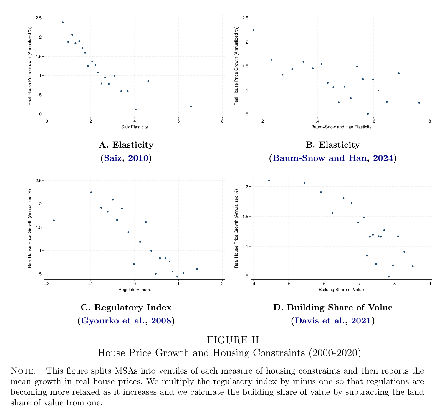
If housing constraints are the central factor determining the growth in house prices, then housing quantities should reflect the inverse relationship. Ceteris paribus, cities with relatively unconstrained housing markets should build more housing, thus suppressing growth in house prices. Figure III checks if this is the case by plotting the total annualized growth in housing quantities against the same measures of housing constraints. The results are not consistent with this argument. All of the measures but the building share of land value are at least weakly negatively correlated with housing quantities. It is clear that none of these measures is strongly positively correlated with growth in housing quantities, as would be the case if most of the variation in house price growth were explained by variation in the growth of housing quantities (that is, explained by differential supply elasticities).
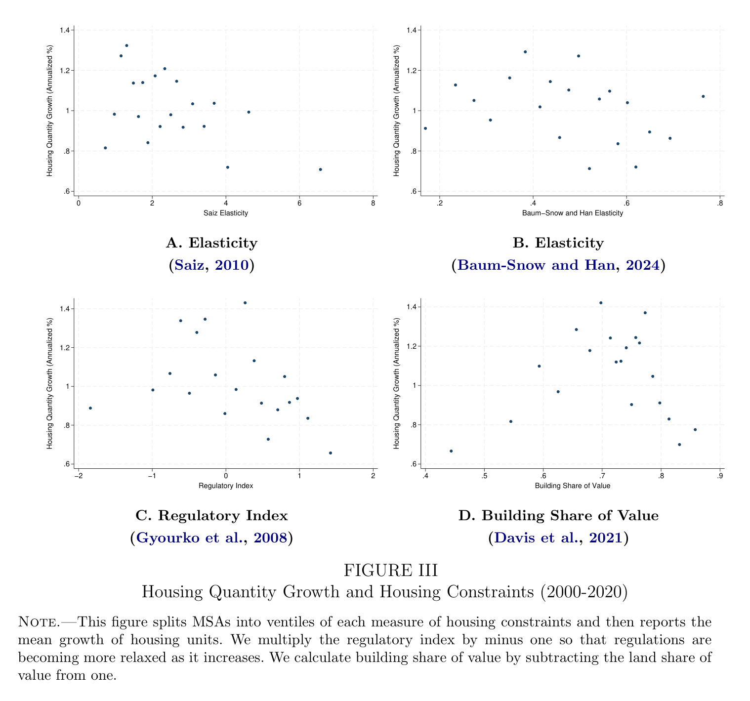
The empirical section opens by reproducing the other side's best chart. Sort metros into twenty bins by each constraint measure, plot price growth: constrained cities unmistakably got more expensive. On the Saiz measure, moving across the range takes real price growth from over 2% a year to under 0.5%—roughly 50% versus 10% cumulative over two decades. This is the correlation the entire deregulation movement stands on, confirmed in the paper's own data. Starting here is a choice: the authors are establishing that they see what everyone sees before arguing about what it means.
Then the first crack. If the price pattern came from supply rigidity, quantities should mirror it—unconstrained cities should be building conspicuously more. The equivalent chart for building shows they aren't: quantity growth is flat-to-negative across the constraint measures. Two charts, built the same way from the same data, telling incompatible stories: prices say constraints matter, building says they don't. A supply explanation needs both charts to cooperate. Everything that follows is about which chart is telling the truth about supply—and the authors will argue it's the building chart, because prices have another way of rising that building does not.
Of course, a critical step in this argument is that shocks to demand and supply are held constant when comparing cities with different elasticities. As demonstrated by Davidoff (2016)Supply Constraints Are Not Valid Instrumental Variables for Home Prices (Critical Finance Review 2016)Shows the standard constraint measures are 'correlated with many demand factors'—education, immigration, industry mix—so regulated coastal markets are expensive partly because they are desirable and productive, invalidating constraints as instruments.Paper → and Howard and Liebersohn (2021)Why Is the Rent So Darn High? (Journal of Urban Economics 2021)Builds a new rent index and finds the effect of income growth on rents is independent of measured supply elasticity, attributing this to strong migration responses—rising demand to live in inelastic cities drives rents everywhere.Paper →, local elasticity measures are strongly correlated with differences in housing demand. For example, coastal California has, in addition to restrictive zoning and difficult terrain, pleasant weather and excellent Mexican food, both of which increase housing demand. Therefore, it is difficult to disentangle the effect of housing constraints from high demand.
Figure IV plots house price growth against the growth in house quantities. We see a strong positive relationship between growth in house prices and quantities: cities that experienced large growth in house prices are generally cities that experienced large growth in housing quantities, consistent with Davidoff (2013)Supply Elasticity and the Housing Cycle of the 2000s (Real Estate Economics 2013)The 2000s boom-bust was not larger in supply-inelastic regions once demand is accounted for; the regions with the biggest cycles also built the most.Paper →. This picture suggests that differential shifts in demand are important drivers of housing market dynamics. Of course, it does not indicate that differences in supply constraints are irrelevant, just that it is important to condition on demand when examining the effects of housing constraints on house price growth.
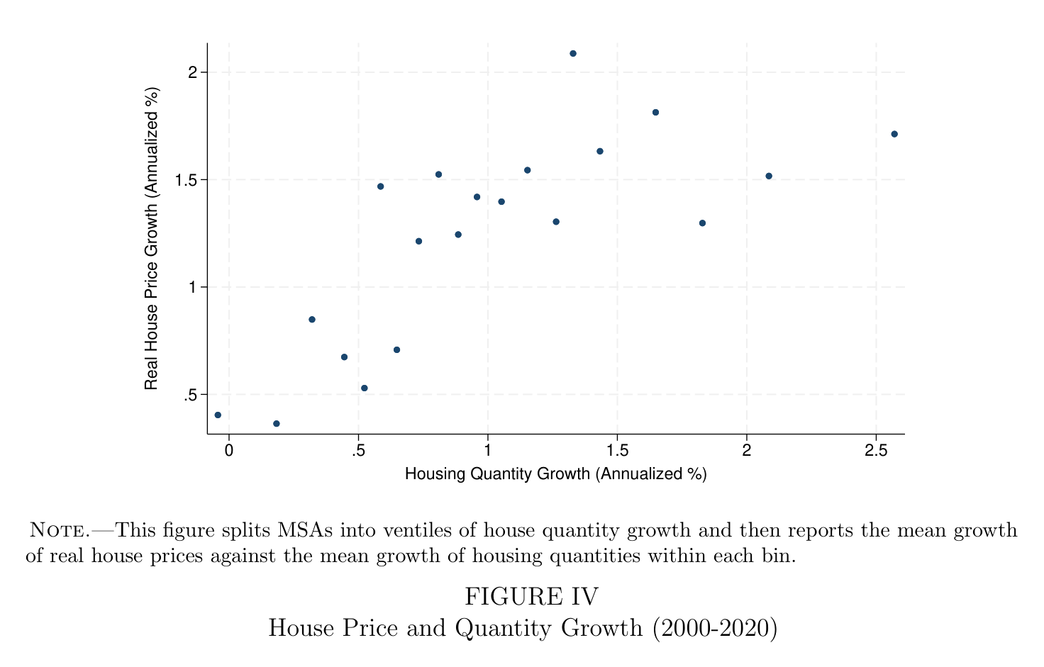
Why can that famous chart not settle anything? The authors answer in their own words: "As demonstrated by Davidoff (2016)Supply Constraints Are Not Valid Instrumental Variables for Home Prices (Critical Finance Review 2016)Shows the standard constraint measures are 'correlated with many demand factors'—education, immigration, industry mix—so regulated coastal markets are expensive partly because they are desirable and productive, invalidating constraints as instruments.Paper → and Howard and Liebersohn (2021)Why Is the Rent So Darn High? (Journal of Urban Economics 2021)Builds a new rent index and finds the effect of income growth on rents is independent of measured supply elasticity, attributing this to strong migration responses—rising demand to live in inelastic cities drives rents everywhere.Paper →, local elasticity measures are strongly correlated with differences in housing demand. For example, coastal California has, in addition to restrictive zoning and difficult terrain, pleasant weather and excellent Mexican food, both of which increase housing demand." The joke is the argument. The same coasts and mountains that make building hard make living desirable, so the constraint measures double as desirability measures—and constrained-and-expensive is what you'd observe whether constraints matter or not. (A footnote adds that the fish tacos in San Diego are particularly tasty. The paper's sense of humor concentrates at exactly its most important analytical points.)
The supporting chart clinches it: across cities, price growth and quantity growth are strongly positively correlated—the places that built the most also saw prices rise most. Think about what that means. If cities mainly differed in supply, the correlation would be negative: big supply means lots of homes and cheap ones. A positive correlation means cities mainly differ in demand—demand pushes prices and building up together. So the cross-section of American cities is demand variation nearly everywhere you look, and any honest test of supply differences has to hold demand fixed first. Which is precisely the design of the tests that follow.
Figure V takes this approach by plotting growth in house prices for each measure of housing constraints against growth in total income separately for MSAs with above and below median values of each constraint measure. Dividing cities in this way is consistent with previous work of Glaeser et al. (2006)Why Have Housing Prices Gone Up? / Urban Growth and Housing Supply (2005-06)Founding papers of the regulation view: house prices increasingly exceed construction costs in regulated markets, and the gap is attributed to regulatory barriers—the 'regulatory tax.'Paper → and Ganong and Shoag (2017)Why Has Regional Income Convergence Declined? (JUE 2017)Argues housing constraints broke the century-old pattern of poor states catching up to rich ones, by pricing low-skill workers out of high-income places.Paper →. As discussed in Section 2, for the same growth in housing demand MSAs with unconstrained housing markets should show relatively less growth in house prices compared to MSAs with constrained housing markets. Across every measure, we find that house prices for more- and less-constrained cities have the same slope with respect to changes in income growth. To the extent that changes in income growth reflect different demand conditions, these pictures show that none of the measures of supply constraints translate into differences in price growth.
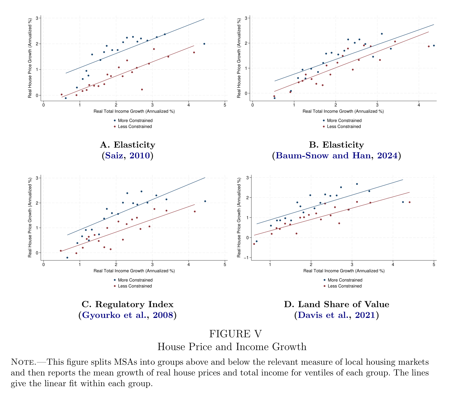
The fact that supply constraints do not affect the relationship between income and house price growth is not consistent with the logic of how different housing supply elasticities affect house prices given in Equation (4). But this result could be consistent with the important class of local labor market models where migration across cities is driven by the cost of housing relative to income (Moretti, 2011Local Labor Markets (Handbook chapter, 2011)The standard framework for how workers move between cities in response to wages, amenities and housing costs—the model class in which migration can equalize price-to-income ratios.Paper →). At the extreme, it is possible that migration causes price-to-income ratios to be equalized so that local housing supply elasticities will have zero effect on prices but large effects on migration and the quantity of housing (Aura and Davidoff, 2008Supply Constraints and Housing Prices (Economics Letters 2008)A calibrated model in which even large local supply expansions barely move prices, because migration and demand from outside the region absorb them—relaxing one city's constraints does little.Paper →; Howard and Liebersohn, 2021Why Is the Rent So Darn High? (Journal of Urban Economics 2021)Builds a new rent index and finds the effect of income growth on rents is independent of measured supply elasticity, attributing this to strong migration responses—rising demand to live in inelastic cities drives rents everywhere.Paper →). In our framework this would be reflected as the price elasticity of demand (ϵ) being very large in Equation (4). Alternatively, income growth may be correlated with positive housing demand shocks in more elastic cities, which would make house price growth in those cities look similar to less elastic cities. Both theories imply that income growth predicts large differences in quantity growth across more and less elastic cities.
This is the central price test. Plot price growth against income growth separately for the constrained and unconstrained halves: the standard view predicts a steeper line for constrained cities—more price per unit of demand. Instead the slopes are the same, on every one of the four measures. For the same growth in demand, constrained cities' prices rose no faster.
Then the authors steel-man their own result, naming two serious theories under which equal price slopes could occur even if elasticities genuinely differed. The first: migration arbitrage. In local labor market models (Moretti), people move between cities based on housing costs relative to incomes. Push that to its extreme and migration becomes a great equalizer—if a constrained city's prices outrun incomes, people leave until the ratio snaps back. In that world, elasticity has "zero effect on prices but large effects on migration and the quantity of housing": a constrained city doesn't get higher prices, it gets fewer people. Equal price slopes would then be an artifact of population flows, not evidence about supply curves. (The citations—Aura and Davidoff, Howard and Liebersohn—mark this as the location-demand school's home ground; these are authors whose work usually supports the paper's side of the debate, here treated as the source of the threat.) The second: correlated demand shocks—elastic cities' income growth arrives bundled with extra hidden demand, inflating their price growth until it matches the constrained cities'.
Both theories fail on the same margin, as the closing sentence states: each rescues equal prices only by predicting unequal quantities. Migration arbitrage means elastic cities absorb large population inflows and build accordingly; correlated shocks mean the hidden demand must show up as extra construction. "Both theories imply that income growth predicts large differences in quantity growth across more and less elastic cities." So the price evidence alone settles nothing—by the authors' own admission—and everything now rides on the building chart. A footnote adds that the migration story is self-undermining anyway: for migration to equalize prices, supply must be highly elastic everywhere to absorb the flows, which concedes the conclusion.
In Figure VI, we check if housing constraints affect the relationship between growth in housing quantities and income growth. Since growth in total income reflects growth in population as well as growth in average income there will be a tight relationship between housing quantities and total income growth. But if the migration mechanism is important, then relatively unconstrained cities should see more growth in housing quantities for the same change in total income compared to relatively constrained cities. These figures show that this is not the case. Across all of the measures of constraints, relatively constrained cities show the same growth in housing quantities in response to higher income growth as relatively unconstrained cities. Interestingly, there is not even a gap in the average housing quantity growth across the two types of cities, which means the price gap or “intercept” is difficult for the standard model to reconcile (Section A2).
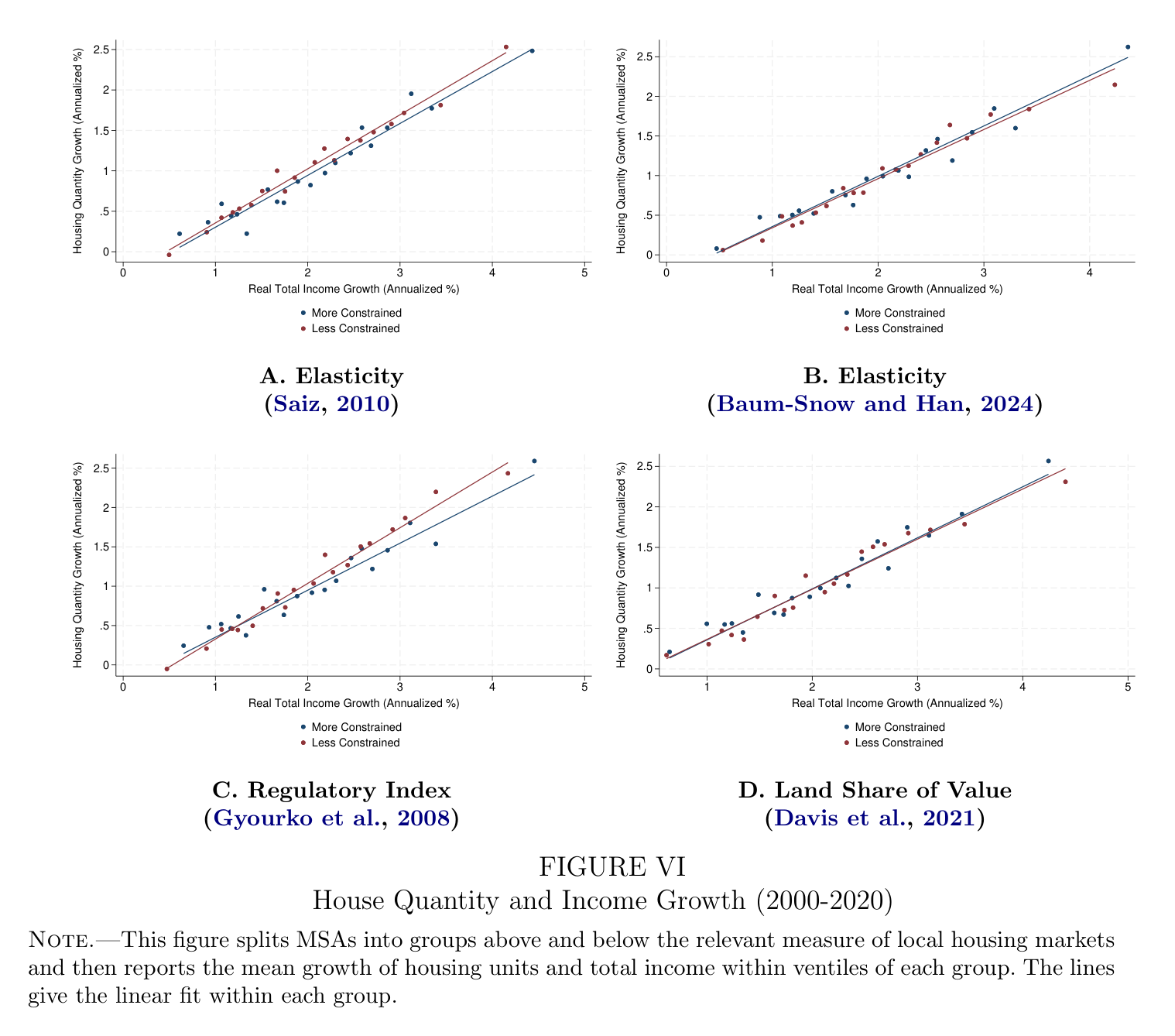
Through the lens of the housing demand-and-supply model in Section 2, these figures imply that differences in housing supply elasticities across cities are quantitatively not important for explaining how income growth, or housing demand growth more generally, affects differences in house price and house quantity growth. But perhaps income growth is a very specific measure of housing demand and more representative measures of housing demand show different results. To check on this concern, Figure VII plots house price growth against house quantity growth, which means that the slopes are the inverse elasticities of housing supply (Saiz, 2010The Geographic Determinants of Housing Supply (QJE 2010)The field's standard supply-elasticity estimates: satellite measures of water and steep slopes, combined with regulation, yield an elasticity for every metro. Miami, LA, SF, NY, Boston, Chicago and Seattle rank among the most inelastic; Houston, Austin, Charlotte, Kansas City and Indianapolis among the most elastic.Paper →), P̂ = 1/ψ Ĥ , when there are no confounding supply shocks. In this case, these figures will trace out different loci for cities with high and low elasticities. These figures confirm that there is no evidence that these less constrained cities tend to have relatively higher elasticities of supply, even in the unconditional relationships between housing prices and quantities. While the Baum-Snow and Han (2024)The Microgeography of Housing Supply (JPE 2024)Modern supply-elasticity estimates built from neighborhood-level data—one of LMW's four constraint measures.Paper → slopes appear to be slightly distinct across the two groups of cities, the higher slope among less-constrained cities is actually the opposite of what the standard model would predict (that is, the figure suggests cities that should have more-elastic housing supply actually have less-elastic housing supply).
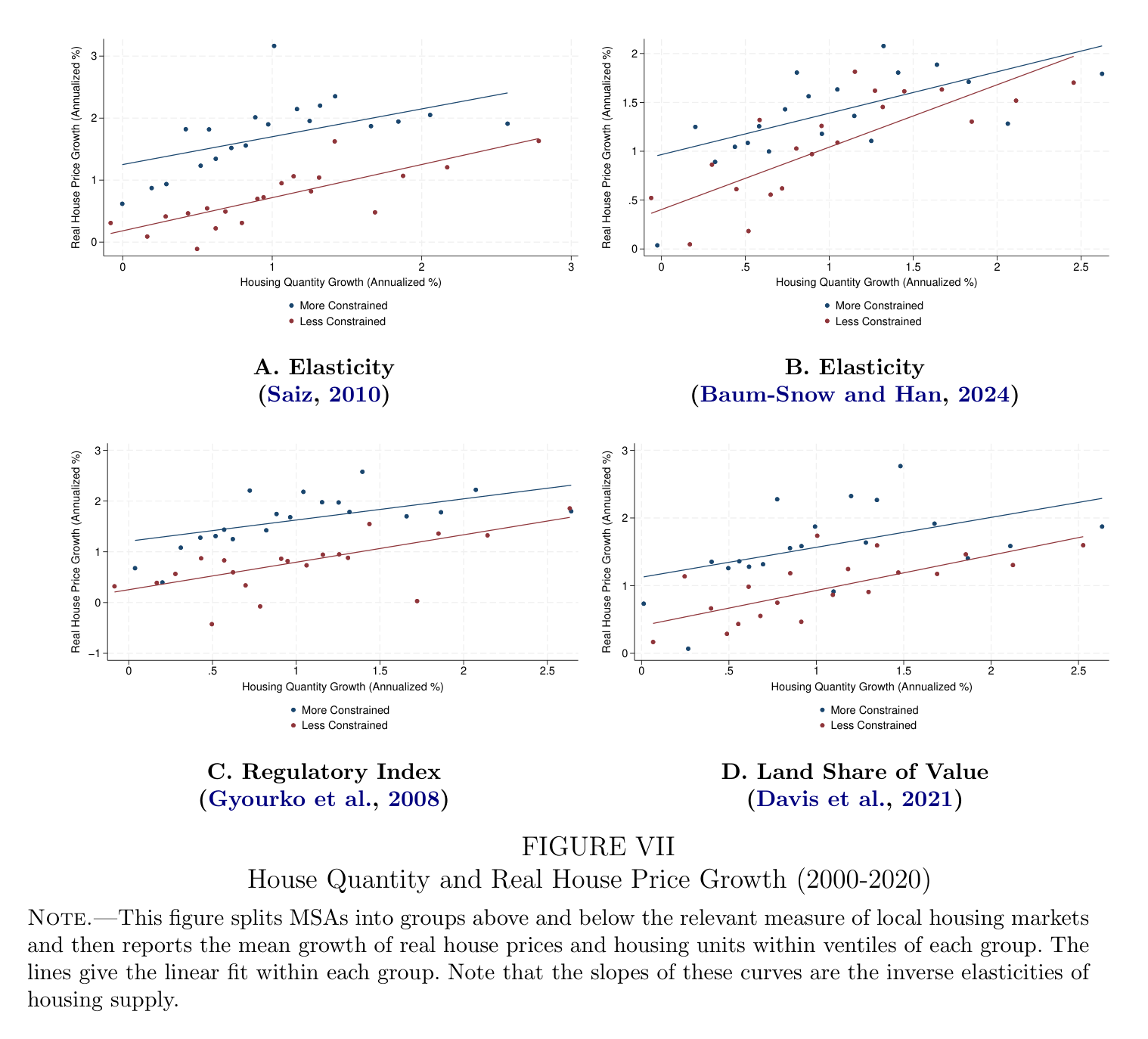
These results highlight that from the perspective of the standard model, it is entirely legitimate to test for differential supply elasticities by regressing prices on quantities. The only threat to identifying different supply elasticities in this way comes from differential distribution of housing supply shocks across groups of cities. However, we focus on variation correlated with income growth for several reasons. First, it is possible that even in the standard model different kinds of demand shifters will have different treatment effects on the response of housing units relative to house prices (see Section A2 and Louie et al. (2025c)LMW, Response to FurthThe point-by-point reply—on this page. Click to open the tab.Open tab →). By conditioning on specific measures of demand like total income, per capita, and population growth, all of which are strongly correlated with housing market outcomes, we increase the likelihood that we will be recovering uniform treatment effects across cities. Second, by conditioning on income growth we raise the empirical hurdle in order for supply shocks to explain the irrelevance of constraint measures. If we want supply shocks to explain the unconditional correlations in Figure VII, it is necessary for supply shocks to be more important in constrained cities, which would be unexpected based on our discussion in Section 2. But if we condition on income growth it means that it must not only be true that there are more positive supply shocks in constrained cities, but also that supply shocks are more positively correlated with income growth in constrained cities. Thus, to rescue differential housing supply elasticities it is necessary to believe that the most constrained, high-growth cities actually experience the largest improvements in housing productivity. This is even less plausible than the possibility of differential likelihoods of supply shocks on average. Finally, by documenting the correlations of income growth and its components with housing market outcomes, we hope to shed light on important empirical moments that can be used to guide research on the housing market going forward.
This is the building test, which the previous passage made decisive. Quantity growth against income growth, by group: the same slope, and—unlike prices—no gap of any kind. Both rival theories needed elastic cities to build conspicuously more per unit of income growth. They don't. Through the model, both margins responding identically means the supply elasticities are effectively the same—or differ in ways none of the four measures can see.
The methodological paragraph then explains why conditioning on income growth was the right design, and it contains the argument's strongest point. Conditioning on income also narrows what a supply-shock story is allowed to claim: to explain these results, supply shocks would now need to be not merely more common in constrained cities but more correlated with income growth there—meaning the most constrained, fastest-growing cities systematically enjoyed the biggest construction-productivity improvements. Each alternative, once inspected, requires believing something stranger than the finding it was meant to overturn. That is the paper's recurring move, and by this point the reader has seen it enough times to anticipate it.
It is also true that relatively constrained cities tend to have higher house price growth on average, as shown by the vertical gap between the two sets of cities in Figure V and Figure VII, but no such gap exists for housing quantity growth in Figure VI. We show in Section A2 that because this “intercept” term only exists for prices and not quantities, it is only consistent with differential supply elasticities if one assumes a set of ad hoc and implausible housing supply shocks: if we take the Saiz (2010)The Geographic Determinants of Housing Supply (QJE 2010)The field's standard supply-elasticity estimates: satellite measures of water and steep slopes, combined with regulation, yield an elasticity for every metro. Miami, LA, SF, NY, Boston, Chicago and Seattle rank among the most inelastic; Houston, Austin, Charlotte, Kansas City and Indianapolis among the most elastic.Paper → elasticities at face value, then on average supply shocks must have increased housing supply in elastic cities by one percentage point per year and reduced housing supply in inelastic cities by one percentage point per year. For comparison, the housing stock grows on average by one percentage point per year. Under this interpretation it is differences in supply shocks, not differences in supply elasticities that account for differences in house price growth and quantity growth across cities. We argue that it is more plausible that this difference in price growth reflects differential amenity growth correlated with the measured supply elasticity (Davidoff, 2016Supply Constraints Are Not Valid Instrumental Variables for Home Prices (Critical Finance Review 2016)Shows the standard constraint measures are 'correlated with many demand factors'—education, immigration, industry mix—so regulated coastal markets are expensive partly because they are desirable and productive, invalidating constraints as instruments.Paper →) and limitations in how well price indexes adjust for changes in housing quality or local amenity valuation, both of which will be priced in any standard housing model (Harding, Rosenthal and Sirmans, 2007Depreciation of Housing Capital, Maintenance, and House Price Inflation (JUE 2007)Repeat-sales estimates of housing depreciation and maintenance—evidence that housing quality changes over time and is priced, which matters for LMW's quality margin.Paper →; Billings, 2015Hedonic Amenity Valuation and Housing Renovations (Real Estate Economics 2015)Renovations are capitalized into house prices—evidence that investment in quality shows up as measured price growth.Paper →; Diamond, 2016The Determinants and Welfare Implications of US Workers' Diverging Location Choices (AER 2016)Cities attracting educated workers develop better amenities endogenously—the mechanism by which rising demand makes places nicer, which price indexes then record as price growth.Paper →).
In short, none of the figures suggest an important role for housing supply constraints in explaining house price growth and quantity growth in a way that the supply-centric view predicts. We next confirm this insight in regression form and show that it is a robust conclusion.
The authors volunteer the fact their critics will spend the next year attacking. At any given level of income growth, constrained cities' prices still grew faster—the fitted lines are parallel, but the constrained line sits higher. They name it the "intercept," and everything contentious about this paper lives in it: Armlovich's viral thread, the sharpest sections of Furth's responseFurth (2025), Response“supply and demand shocks together lead to systematically higher prices in more-constrained metros, but do not lead to any differences in quantities. That can only happen via systematically larger demand shocks and smaller supply shocks in more-constrained metros.”Open in context →, the FAQLMW FAQ, Q14“this correlation actually points to implausibly large, ad hoc shifts in housing supply functions.”Open in context →'s longest answers.
Their reply, compressed here and expanded in an appendix, has two steps. First, the gap exists "for prices and not quantities"—constrained cities collected extra price growth without any corresponding shortfall in building. A supply-side story cannot do that: rigidity raises prices by blocking homes, so a price gap with no building gap requires an implausible combination of shifts—supply curves in elastic cities shifting outward by amounts comparable to all the housing they built over the period. Second, whatever produces the gap must therefore move prices while leaving quantities alone, and their candidate is demand for quality: amenity values and housing improvements that even repeat-sales indexes record as price growth.
Note the structure of the move—concede the fact, show the rival explanation is arithmetically absurd, offer an interpretation. The concession is genuine and the arithmetic is strong; the interpretation is the paper's softest joint, resting on imperfectly measured quality rather than anything directly observed. The authors know this—it is why Section 5 and a dedicated appendix exist—and it is the honest place for a skeptical reader to push.
We estimate the following regressions:
The coefficients of interest are β and γ, which recover the differential response of house price growth and house quantity growth to income growth for cities that have relatively more elastic housing supply. In terms of our discussion in Section 2, β = β −β and γ = γ −γ. Thus, we expect β < 0 and γ > 0, or that cities with relatively more elastic housing supply experience relatively less price growth and more house quantity growth for the same income growth. In contrast, we find that the coefficients are small, statistically insignificant, and often of the wrong sign, which implies that differences in housing supply are quantitatively not important for explaining differences in house price and quantity growth across cities (Section 2). In Section 4.4 we discuss the robustness of our results to more flexible discretizations or using a continuous specification.
Table II reports the results for the Corelogic house price index where panel A uses total income growth, our preferred measure of demand. Total income growth is strongly correlated with house price growth: a one percentage point increase in total income growth predicts a 50-60 basis point increase in house price growth. However, the interaction term of total income growth with the housing supply constraint indicator is essentially zero and statistically insignificant across all measures of the elasticity.
One concern might be that we are using total income growth when we should be using only growth in per capita income or only growth in population as our measures of housing demand. We show in Section A1 that total income is a legitimate measure of housing demand in standard models, and in Louie et al. (2025c)LMW, Response to FurthThe point-by-point reply—on this page. Click to open the tab.Open tab → we show that it is appropriate even in a relatively non-standard model. The intuition is that our empirical approach only depends on the structure of the housing market and is independent of any assumptions about migration. Even so, by checking if the results depend on the measure of growth we can also determine if it is plausible for supply shocks to be more important in more constrained areas (see Section 2). Table II panel B shows that per capita income growth is strongly correlated with growth in house prices and this correlation is identical across more- and less-constrained MSAs for every measure of constraints. Interestingly, the correlation of per capita income growth with prices is somewhat stronger than the correlation of total income growth with prices. Panel C turns to population growth and, while the correlation between population growth and price growth is somewhat smaller, we again find that this correlation is unaffected by whether or not a city appears to be supply constrained. Table A2 repeats these regressions for growth in the median home value and finds the same results. There is no evidence that using total income as a regressor is affecting our results one way or another. Given these results, we use total income growth as our baseline regressor, but in Section 4.4 we repeat our quantity results using per capita and population growth as robustness checks. Importantly, the fact that all of the specifications show the same non-result is inconsistent with the hypothesis that supply shocks are more important in more constrained areas.
These are the same results as the figures, now with standard errors. Price growth is regressed on income growth, the less-constrained indicator, and their interaction: income growth strongly predicts price growth, and the interaction—the entire question in one coefficient—is statistically and economically nothing, on all four constraint measures.
Then a robustness check that doubles as a diagnosis. Rerun everything with per-capita income as the demand measure; rerun with population. Same null, every time. This matters beyond thoroughness, because the framework showed that if supply shocks were contaminating the results, the three demand measures would disagree—per-capita income loads least on the contaminated channel, population the most. Their unanimity is the fingerprint of a clean result. It also pre-answers the most common objection the paper would face—"total income is the wrong demand measure"—with the objector's own preferred variables. Any critic who wants to attack the demand measure must now explain why every version of it produces the same answer.
Table III changes the outcome variable to housing quantity growth. Panel A uses the growth in the number of housing units and panel B uses population growth. Across all of the specifications only the regulatory index seems to slighty raise the positive effect of income growth on growth in housing units and population. Even taking this small effect at face value, the fact that Table II showed that there is essentially no effect on prices as one would expect from a supply-centric view, suggests this result is likely spurious and below we confirm that this effect disappears once we exclude low-growth cities. The Saiz, Baum-Snow and Han, and building share of value measures all have no effect on the correlation between quantities and income growth and mostly have the wrong sign. Overall, we find little to no evidence for relatively more growth in housing quantities in less constrained areas for any of the constraint measures. Similarly, the coefficient on the indicator itself is not significantly or even consistently positive. So while less-constrained cities tend to have lower house price growth on average in some specifications, they do not tend to have more growth in housing units or population, inconsistent with the basic supply-side mechanism (see Section A2).
Panel C uses the change in the average number of rooms per person as an alternative measure of housing quantity outcomes. If housing markets are responding on the intensive margin (for example, larger homes) more than the extensive margin (more homes) then this variable should capture some of the differential response. Here total income growth is negatively correlated with the change in rooms per person, suggesting that cities that are growing become more crowded or less spacious, perhaps as households opt to live closer to certain amenities associated with higher density. But this correlation is completely unaffected by the measure of housing constraints. Given differences in income growth, having a housing market that is ostensibly more or less constrained does not affect differences in the quantity of housing per person.
Together these results show that neither prices nor quantities exhibit the kind of differential correlation with income growth that we would expect if housing supply constraints are actually different across these groups. To summarize this point, we estimate instrumental variable specifications along the lines of (7), where we interact growth in house prices with the indicator for being less constrained and then instrument for that variable with total income growth interacted with the same indicator. This allows us to estimate the supply elasticity directly and focuses the threats to identification on just differential correlations between supply shocks and income growth.
Table IV reports estimates for growth in the quantity of housing with panel A using the house price index and panel B using the median home value. The coefficients on price growth give the estimated elasticities of housing quantity with respect to price growth for each type of city. We report the chi-squared test for rejecting the hypothesis that the estimated elasticities across more- and less-constrained cities are the same. We also report the first-stage F-statistics for each group of cities when estimated separately to explicitly verify that the instrument is strongly correlated with house price growth. In none of the specifications can we reject that the elasticities are equal at standard levels of significance. Only the regulatory index displays a lower supply elasticity in more constrained cities that is at least somewhat economically meaningful. But the difference in the relationship is simply quantitatively too small and imprecise to be able to say that less regulated cities have a meaningfully different response in the quantity of housing units, and robustness checks below show that this estimate is not robust to dropping low-growth cities.
Table A3 runs the regressions replacing housing unit growth with population growth and finds essentially the same results. We do not find any evidence that supply constraints are economically or statistically significant determinants of variation in the growth of house prices relative to population.
This passage runs three tests, in rising order of directness. First, the building version of the benchmark regression: income growth predicts quantity growth tightly—this is the strongest relationship in the paper, with total demand explaining most of the cross-city variation in building—and the constraint measures shift nothing.
Second, a subtler margin: rooms per person. If constrained cities can't add units, their growth should show up as crowding—people squeezing into the existing stock. Growing cities do get slightly more crowded, but identically in constrained and unconstrained cities. Even on the intensive margin, the constraint measures fail to matter.
Third, the most direct test the framework allows: estimate the supply elasticity itself. Instrument prices with income growth and measure how much building a given price rise elicits, separately for each group of cities. This is the exact quantity the entire literature claims to measure—Saiz's rankings are estimates of it—and the estimates come out statistically indistinguishable across groups in every specification. One partial exception is reported honestly because critics cite it: on the Wharton regulation index, constrained cities show a somewhat lower elasticity, but the difference is small, imprecise, and vanishes when slow-growing cities—where constraints shouldn't bind anyway—are dropped. Replacing units with population growth changes nothing. The chapter's conclusion in one line: measured directly, on their own definition, the supply curves of NIMBY and YIMBY America have the same slope.
We argue that our analysis is particularly attractive because we do not require exogenous variation in housing demand to evaluate if differences in housing supply elasticities across U.S. cities explain differences in house price and quantity growth (Section 2). But exogenous variation can help distinguish between the explanation that supply elasticities are not different, at least as conventionally measured, and the alternative that differentially correlated supply shocks render actual differences in supply elasticities uninformative about city house price and quantity growth. We distinguish between these explanations using two distinct approaches. First, we use three standard instruments for housing demand to re-estimate our housing supply elasticities. As explained in Section 3, these are a Bartik instrument for labor demand, July humidity, and January temperature. Second, we exploit the shock to housing demand due to the shift to work-from-home from Mondragon and Wieland (2025)Housing Demand and Remote Work (NBER WP)Establishes pre-pandemic remote-work exposure as a valid, plausibly exogenous shifter of post-2020 housing demand—the instrument behind LMW's cleanest causal test.Paper →, who show that it is a plausibly exogenous shock to local housing demand. Both of these exercises recover little difference in supply elasticities across cities, consistent with our non-causal evidence. In addition to providing plausibly exogenous variation, these shocks are useful because we do not condition on changes in total income, per capita, or population growth, allowing us to sidestep any concerns about how those variables may be affecting our analysis.
Table V presents the results using the standard instruments. In six of the eight specifications it is the more-constrained cities that are estimated to have more elastic housing supply functions, with an economically large and statistically-significant difference for column two of panel A. These results are the opposite of the standard view. While the estimates using the regulatory index point in the standard direction, these results again disappear after dropping low-growth cities. Therefore, even when using standard approaches to isolating housing demand that do not rely at all on our measures of income growth we find that supply elasticities do not appear to be different across cities. These regressions return elasticities that are generally lower than what we find using total income growth as an instrument, which could be consistent with supply shocks biasing the income-based estimates of the supply elasticity upward. For our purposes it is sufficient to document that these elasticity estimates do not suggest that standard measures of housing supply constraints help explain house price or quantity growth across cities.
In our second exercise, we construct a measure of exposure to the rise of WFH over the pandemic, the the employment share of WFH from 2015-2019, which Mondragon and Wieland (2025)Housing Demand and Remote Work (NBER WP)Establishes pre-pandemic remote-work exposure as a valid, plausibly exogenous shifter of post-2020 housing demand—the instrument behind LMW's cleanest causal test.Paper → show is strongly correlated with the increase in WFH over the pandemic and plausibly exogenous. We then interact this measure with each of the indicators for being less constrained (above median). We measure outcomes from 2019 to 2023, the most recent year for which we can measure total income growth.
Because this is a single shock, we present the reduced form results in Table VI to parallel our baseline analysis. In panel A we put total income growth as the outcome to check if growth in more- and less-constrained cities loads equally on the WFH shock. We see some evidence that growth is higher in places that are less regulated, implying there is some heterogeneity in the treatment effect. This heterogeneous treatment effect is not informative about the role of supply constraints in the housing market, but it is important for scaling the demand shock across these different cities. Panel B turns to house prices and finds that remote work does increase house prices, but there is no evidence that house prices grew less in cities that were less constrained. The one statistically significant estimate, on the regulatory constraint, has the wrong sign. Finally, panel C looks at the cumulative growth in the number of units permitted. We use permitted units instead of actual units because the quantity of housing measure we use in other specifications is only available in census years. These estimates show that the increase in housing demand due to WFH had a large effect on permit growth, about two to three times larger than that on house prices. This larger response is intuitive since permits represent the response of housing investment, which is smaller and more volatile than the overall stock of housing. The interaction terms are all positive, sometimes with large coefficients, but the standard errors are far too large to distinguish these estimates from zero. These large coefficients on the interactions are actually due to outliers as quantile regressions, which are less sensitive to outliers than OLS regression, are reported in Table A4 and show that these estimates largely disappear. Critically, none of the measures gives the expected set of coefficients showing relatively less house price growth and relatively more permitting growth in elastic cities in response to the shift in demand.
In short, even when using exogenous variation the measures of housing constraints do not affect the relative growth of house prices and house quantities across cities. We again conclude that differences in housing supply elasticities are quantitatively unimportant for explaining differences in house price and house quantity growth.
Here is the promised causal evidence, for readers who never trusted the correlations—and the results are stranger than a simple confirmation.
With the standard instruments of the literature (Bartik industry shocks, climate), the estimates don't just fail to support the standard view; they point the wrong way. In six of eight specifications, the constrained cities are estimated to have more elastic supply—with one statistically significant reversal. The lone result pointing the standard direction, on the regulation index, dies when slow-growing cities are dropped. If you believed these instruments—and much of the literature is built on them—you would conclude that America's constrained cities are its most flexible builders. The saner reading, which the authors take, is that no version of this evidence supports different elasticities.
Then the cleanest experiment on offer: remote work. The pandemic raised demand wherever WFH-capable jobs concentrated, for reasons unconnected to any city's zoning—and the authors measure exposure with the pre-pandemic WFH share, following Mondragon and Wieland's earlier work establishing the shock's validity. The results, 2019-2023: prices rose with WFH exposure, but no less in unconstrained cities—the one significant interaction has the wrong sign. Permits responded two to three times more strongly than prices, as investment should, but with no credible difference by constraint status; the few large interaction coefficients are outlier artifacts that vanish in quantile regressions. The pattern the standard view demands—less price growth, more building in elastic cities when demand arrives—fails to appear even with demand that is genuinely exogenous. The correlational and causal evidence agree, which was the fourth defense's promise.
In this section we discuss robustness exercises that continue to show that income growth has the same relationship with house price growth and housing quantity growth irrespective of the measured local supply elasticity. In the interests of the reader’s time, we briefly describe them here and relegate a detailed discussion to Section A3. First, we extend the sample to 1980- 2020. Second, we look at just the 1980-2000 subsample. Third, we use quartiles of the housing constraint measure rather than a binary indicator to check if we are obscuring effects in parts of the distributions of constraint measures. Fourth, we use continuous interaction models. Fifth, we exclude cities that are not growing or growing very slowly to make sure we are not biasing the results since housing supply constraints should not be relevant when demand is not increasing or declining. Sixth, we examine growth in rents instead of house prices. Seventh, we examine changes in commuting times. Eighth, we examine housing quantities again but using variation in per capita income growth or in population growth to again address concerns that total income growth somehow biases our results. Finally, we check if our results are being driven by small cities. All of these results continue to show that supply constraints do not explain house price growth and housing quantity growth across cities since at least 1980.
This one paragraph lists nine robustness checks: extend to 1980-2020; the 1980-2000 subsample alone; quartiles instead of halves; continuous interactions; dropping slow-growth cities, where constraints shouldn't bind; rents instead of prices; commuting times; per-capita and population variants for quantities; excluding small cities. The last one matters most: Furth's response would later argue the unconstrained half is padded with small, cheap metros—the median being a place like Lake Charles, Louisiana—so the comparison never confronts the big coastal cities the debate is actually about. This check answers that objectionFurth (2025), Response“In the less-constrained half (for the Saiz metric), the median 2000 population was 184,000 people (Lake Charles, Louisiana).”Open in context → before it was published: restrict to large cities, same null. Whatever this result is, it is not an artifact of any particular way of cutting the data.
If supply constraints do not explain house price and quantity growth across cities, then how do we explain that house prices grew much faster and housing quantities grew much slower in say San Francisco than in Houston (2.4 vs 1% p.a. for prices, 0.6 vs 2.2% p.a. for quantities)? We argue that a model with two housing margins—quantity and quality—helps explain housing outcomes for these cities while also being consistent with other important features of the data. The intuition is the following: Labor demand shocks in San Francisco have tended to raise per capita income (2.2% p.a.), perhaps due to relatively inelastic labor supply, and so raised demand for housing quality, which pushes up prices but has little effect on the demand for housing units. In contrast, labor demand shocks in Houston have tended to increase employment with relatively little gain in per capita incomes (0.8% p.a.). Therefore per capita income, demand for housing quality, and house prices moved relatively little but housing quantities increased substantially. While our exact specification of this idea is simple and somewhat novel, the basic notion that housing is a bundle of attributes that are demanded and supplied goes back to at least Rosen (1974)Hedonic Prices and Implicit Markets (JPE 1974)The hedonic-pricing classic: a house is a bundle of attributes, each implicitly priced—the reason price indexes capture quality as well as scarcity.Paper → and is reflected in the fact that hedonic price adjustments are a first order concern in housing markets (see also Epple, Quintero and Sieg (2020)A New Approach to Estimating Equilibrium Models for Metropolitan Housing Markets (JPE 2020)Estimates an equilibrium model in which housing is produced and consumed in quality-adjusted units—supporting LMW's point that quality adjustments are first-order in housing markets.Paper → and related work). We are simply demonstrating that the fact that housing markets do not have a single margin of adjustment has fundamental implications for how we try to explain housing market dynamics.
Having spent the paper showing what doesn't explain the cross-section, the authors owe an answer for the pair everyone reaches for. San Francisco's prices grew 2.4% a year against Houston's 1%; Houston built at nearly four times San Francisco's rate (2.2% versus 0.6%). If not supply machinery, what?
Their answer starts in the labor market. San Francisco's economic shocks raised per-capita income—2.2% a year, extraordinary by national standards—while barely adding employment; Houston's shocks added employment and people while barely moving income per person (0.8% a year). And the two kinds of growth buy different things. Income demand is demand for better housing: it bids up prices and adds few units. Population demand is demand for more housing: it gets built. Same underlying supply machinery, different demand arriving in opposite forms, opposite outcomes. The famous pair, on this reading, illustrates the composition of demand—not a difference in what the cities are capable of building.
Note what kind of claim this is. The null result was measurement, defended six ways. This is interpretation—the authors' preferred story about what fills the space the null cleared—and they present it as such, with a model and supporting estimates rather than proof. The distinction between what the paper measures and what it suggests is exactly where honest readers and hostile ones will draw different lines.
In this framework, relative to the standard model of housing supply in Equation (3), there are two housing supply curves, one for housing quality and one for housing quantity: bq = ψ P̂, bu = ψ P̂. where q is housing quality, u is housing quantity (units), ψ and ψ are the respective supply elasticities, and P̂ and P̂ are the respective prices of quality and quantity. We observe the constant-quality price so that the total price change is P̂ = P̂ + P̂. Quality can encompass housing fixtures and house size, but also relatively fixed attributes such as an ocean view or access to specific schools.
In the two-margin model, a housing demand shock that raises the demand for housing quantity moves the housing market along the unit supply curve with elasticity ψ, resulting in higher quantities and prices. In contrast, a housing demand shock that raises only the demand for housing quality raises house prices without increasing quantity, seemingly implying a perfectly inelastic supply of housing quantity despite the true underlying unit elasticity still being ψ. Figure VIII illustrates this situation graphically and shows that because we can only observe the composite price P̂, the market for units will appear to have inelastic supply.
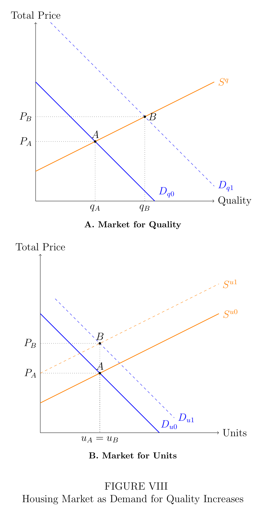
Consistent with this model, we find that per capita income growth and population growth imply very different housing unit supply curves. Table IX shows that the unit supply elasticity in Equation (7) is 0.2 when instrumenting with per capita income and 1.5 when instrumenting with population growth. This is consistent with our results in Table II and Table VII, which show that per capita income growth is strongly correlated with prices but not quantities, and Table VIII which shows that unit growth is strongly correlated with population growth. Furthermore, as the panels in Figure IX show, San Francisco and Houston’s price and quantity growth are almost exactly what one would expect given growth in per capita income and population. Of course, this does not mean that income and population growth explain all variation in prices and quantities. Expectations, wealth, amenities, changing taste, the income distribution and demographics will all affect housing markets in combination with average income and population growth. The key point is that with multiple margins of housing demand, unit supply curves may look very different depending on the composition of demand and irrespective of a city’s regulatory environment.
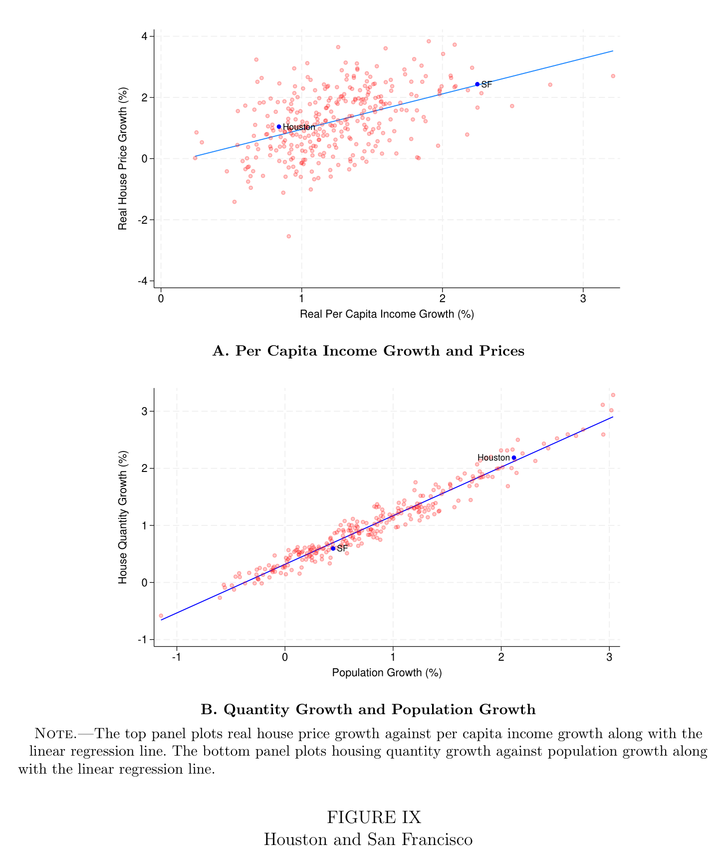
This passage formalizes the interpretation. Housing has two supply curves—one for units, one for quality, where quality spans everything from square footage and finishes to school districts and neighborhood amenity. The price you observe is the sum of both margins' prices, because no index fully separates them: even repeat-sales methods miss renovations between sales and cannot price the changing value of a location at all.
The consequence is the paper's most consequential idea. A demand shock aimed at quality raises measured prices without touching units—"seemingly implying a perfectly inelastic supply of housing" while the unit-supply machinery sits idle and undamaged. A city can look supply-constrained without being supply-constrained, and no amount of staring at price data can tell the difference.
Then the empirical support. Estimate the unit supply elasticity using income-driven demand: 0.2—housing looks nearly rigid. Estimate it on the same cities using population-driven demand: 1.5—housing looks flexible. Same cities, same rules, same twenty years; the measured stiffness of housing supply depends on which kind of demand you probe it with. That is exactly what the two-margin model predicts, and flatly inconsistent with elasticity being a fixed attribute of a city's regulatory environment—which is what every ranking from Saiz to Wharton assumes it is. Figure IX closes the loop on the famous pair: San Francisco's and Houston's prices and quantities are "almost exactly what one would expect given growth in per capita income and population." The authors bound the claim honestly—expectations, wealth, amenities, and demographics matter too—but the sentence with the largest consequences is aimed at the whole measurement tradition: unit supply curves "may look very different depending on the composition of demand and irrespective of a city's regulatory environment."
This paper revisits the standard view that local housing supply constraints explain differences in local house price and quantity growth. We estimate how shifts in income growth and exogenous housing demand shocks translate into changes in house prices and quantities across U.S. cities measured to be more or less constrained in their housing supply. Contrary to prevailing beliefs and influential narratives, our empirical results consistently show that higher income growth predicts similar growth in house prices, rents, housing quantities, population, and living space per person across more and less housing constrained cities. These results imply that differences in housing supply elasticities across U.S. cities are quantitatively not important for explaining differences in house price and quantity growth. Instead, our evidence suggests that housing supply functions are broadly similar across most metro areas despite very different regulatory and geographic environments, challenging the consensus that relaxing regulatory constraints would substantially expand housing quantities and lower prices.
These results call for a reevaluation of our understanding of housing markets and housing supply, echoing the call by DiPasquale (1999)Why Don't We Know More About Housing Supply? (Journal of Real Estate Finance and Economics 1999)The well-known plea for better housing-supply research: economists know far less about supply than demand. LMW close their paper by echoing it.Paper → more than 25 years ago. We think there are a number of potentially fruitful directions going forward. First, the fact that per capita income growth is strongly correlated with price growth but barely correlated with quantity growth points to multiple margins of housing consumption, namely consumption of quality (or amenities) as well as the consumption of units of a given quality. We are pursuing this direction and give examples of this framework in Section A2 and Louie et al. (2025c)LMW, Response to FurthThe point-by-point reply—on this page. Click to open the tab.Open tab →. In this kind of framework, growth in per capita incomes will raise prices because richer households have more income to spend on high-value housing, but this income growth need not induce any growth in units since richer households do not want to consume additional units of housing in the same city. In fact, unevenly distributed income growth may even reduce population growth if the price growth of local services (including housing) caused by income growth at the top prices out lower-income households. Frameworks that only include one margin of housing demand and supply are likely obscuring critical mechanisms in the housing market. Moreover, if multiple margins are an important feature of housing markets, then standard approaches to estimate supply elasticities will generally not recover the objects of interest (see Section A5).
A second promising avenue that we are pursuing focuses on differences in the labor market and labor supply across metro areas. From the perspective of standard labor market models, the difference in house price growth and housing quantities across cities like San Francisco and Houston may reflect important differences in labor supply elasticities. Some cities, like San Francisco, are home to high-productivity jobs where top workers are very difficult to recruit, thus resulting in very high wages. Other cities may also be home to high-productivity industries, but if appropriately-skilled workers in these industries are relatively more plentiful so that labor supply is relatively higher, then there will tend to be less growth in average incomes and more growth in employment and so population. These mechanisms reinforce the core insight of local labor market models, which is that housing and labor markets are fundamentally connected, and indicate that the distribution of productivity gains may be a critical factor for understanding housing market trends.
The summary restates the finding at its honest strength—the results "challenge the consensus that relaxing regulatory constraints would substantially expand housing quantities and lower prices"—and then opens two research directions, each with an uncomfortable implication.
The first is the quality margin, and buried inside it is a provocative hypothesis. Rising per-capita incomes raise prices without adding units because "richer households do not want to consume additional units of housing in the same city"—they want better ones. Then this: unevenly distributed income growth may even reduce population growth, if income gains at the top bid up local prices enough to push lower-income households out. Read that against the standard narrative. In the YIMBY account, displacement happens because regulation blocks the housing that would absorb newcomers. In this hypothesis, displacement is what quality-demand does—rich arrivals price out poorer residents through the bidding itself, zoning or no zoning. It aligns the paper with the inequality school (Buchholz, Storper and coauthors) it cited as allies, and it is offered as a direction, not a finding.
The second road: labor supply. Why did San Francisco's growth arrive as income while Houston's arrived as people? Perhaps because San Francisco's industries need workers who are genuinely scarce—so competition for them shows up as wages—while Houston's industries draw on plentiful labor, so growth shows up as employment. On this view the deep cause of the housing divergence sits in the labor market: the distribution of productivity gains across industries and places decides which cities get rich and which get big, and housing outcomes follow. Neither direction is proven here. Both are bets on where the explanation lives once regulation is set aside—and notice that neither bet, if it pays off, restores the standard view.